
Kinetics
플레이하며 배우기
이 문제들을 풀어 에너지를 얻은 뒤 낚시하고 탐험하세요. 계정이 필요 없어요.
교육자를 위해: Kinetics(Chemistry, AQA)을(를) 위한 바로 쓸 수 있는 수업 슬라이드, 복습 노트, 다이어그램 — 수업에 사용하거나, 학습자들이 실시간 게임으로 즐기는 인터랙티브 클래스 활동으로 진행하세요.
수업 노트
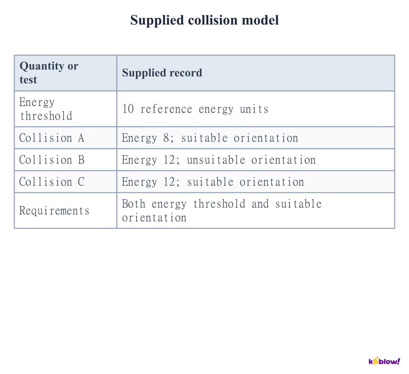
Explain why most collisions do not react
- In the simplified collision model, reacting particles need both sufficient collision energy and a suitable orientation. A collision is not automatically a reaction.
- Increasing collision frequency can increase the number of successful encounters per second without changing the fraction that passes an energy threshold at fixed temperature.
- Use a collision record to distinguish insufficient energy from unsuitable orientation. Energy above a threshold establishes energetic eligibility, not certainty of a successful reaction.
Supplied collision model
Distinguish activation energy from reaction enthalpy
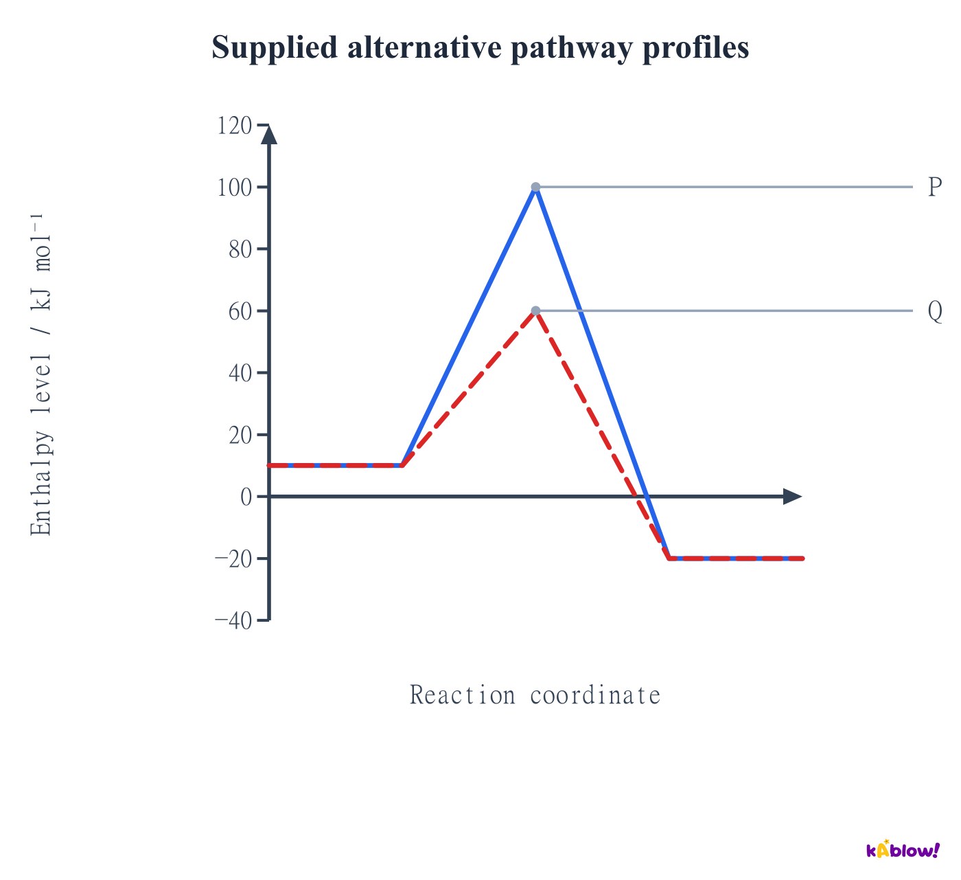
- Activation energy describes the barrier that must be overcome for reaction. A reaction profile compares the barrier with the starting level.
- The reactant–product enthalpy difference does not determine the barrier height for unrelated reactions. An exothermic reaction can have a high barrier and be slow.
- A catalyst changes the pathway and its barrier while leaving the same endpoint enthalpy difference unchanged. The transition state is not an isolable intermediate.
Supplied alternative pathway profiles
Specify a species rate and a reaction rate
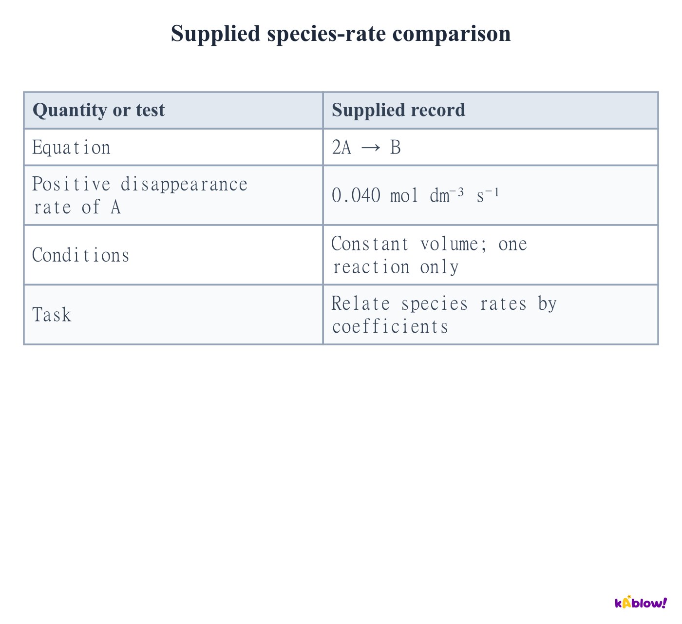
- A species’ formation rate is its concentration increase per unit time. A reactant’s positive disappearance rate is the negative of its concentration gradient.
- For a balanced equation, divide species rates by their stoichiometric coefficients to obtain a common reaction rate at constant volume.
- For 2A → B, A disappears twice as fast as B forms. Do not assign equal species concentration rates merely because they belong to the same reaction.
Supplied species-rate comparison
Calculate an average concentration rate
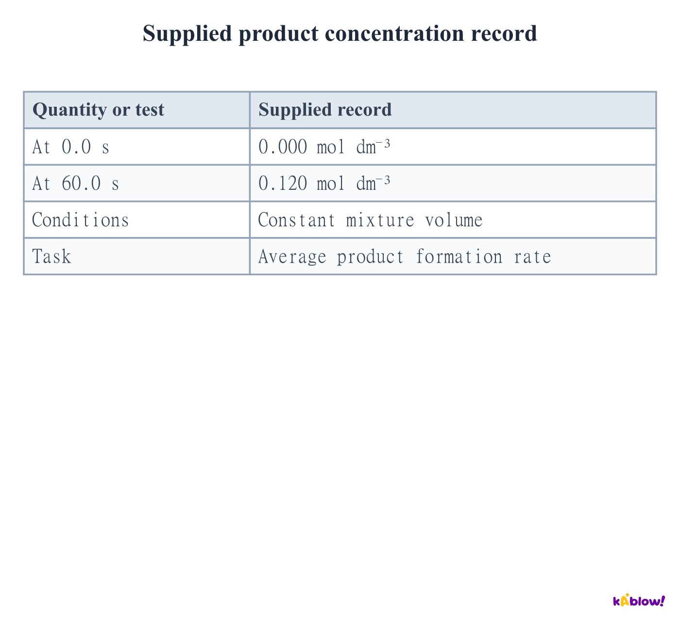
- An average formation rate is the concentration change divided by the elapsed time over a stated interval. Convert minutes to seconds when the requested unit is per second.
- For the supplied product record, the increase from 0.000 to 0.120 mol dm⁻³ over 60.0 s gives 0.00200 mol dm⁻³ s⁻¹.
- This interval average does not determine the instantaneous rate at every moment. Retain the interval and the measured species when stating the result.
Supplied product concentration record
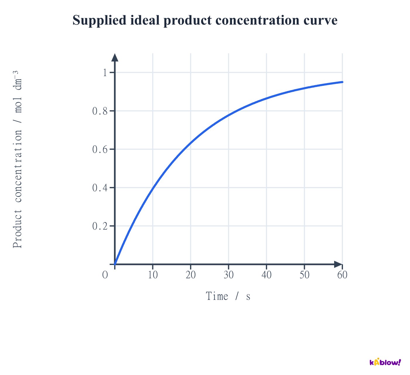
Read an instantaneous rate from a curve
- The gradient of the tangent to a concentration–time curve gives the instantaneous species rate at that time. A secant between two points gives an interval average.
- The supplied idealised product curve rises and becomes less steep. Its positive formation rate decreases in this particular batch model.
- A decreasing rate is not compulsory for every possible reaction. Zero-order behaviour, changing temperature or autocatalysis can give different patterns.
Supplied ideal product concentration curve
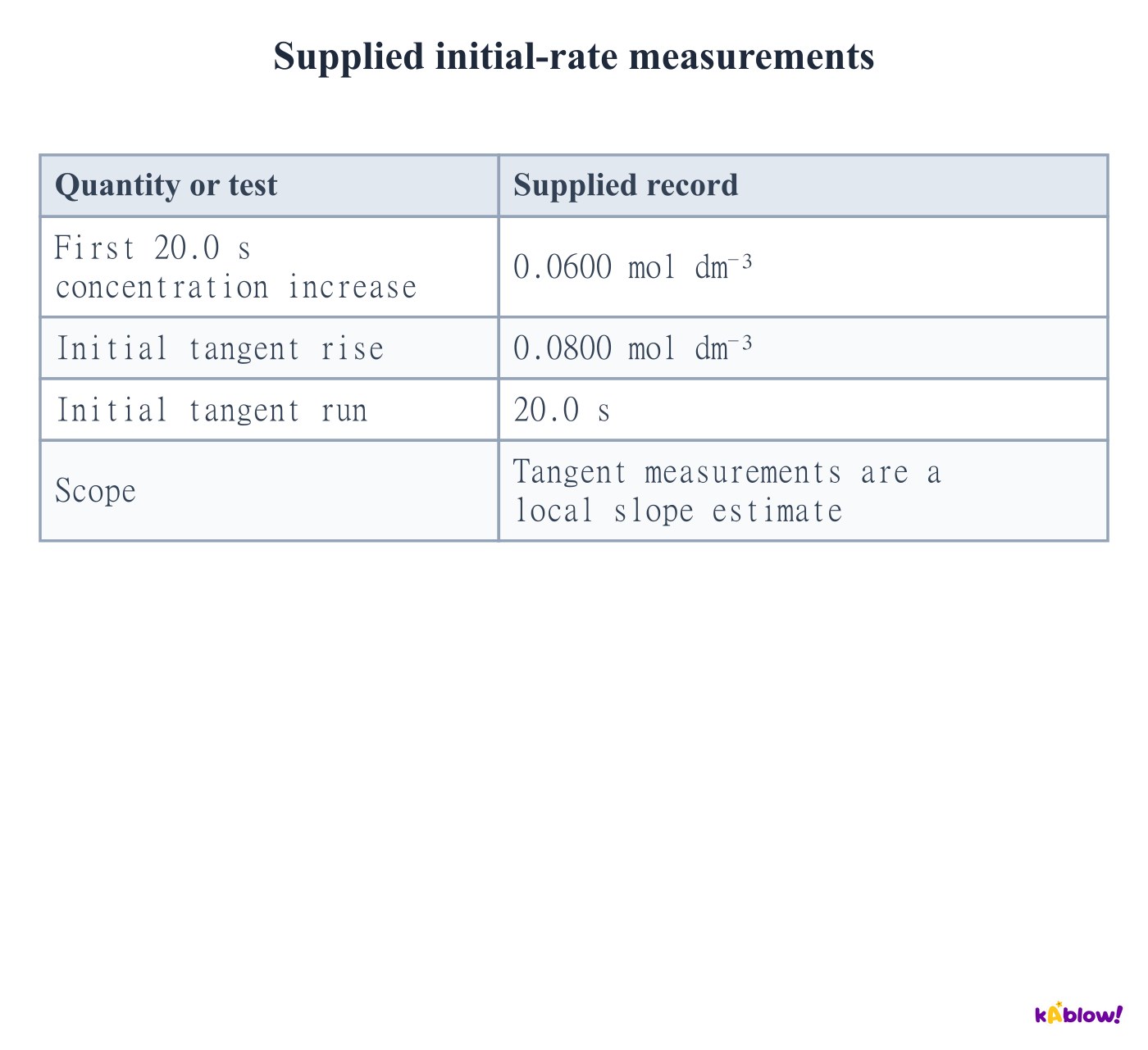
Distinguish initial rate from a first-interval average
- Initial rate is the instantaneous rate at the start, estimated from a tangent or an appropriate initial-rate method.
- A short initial interval can approximate that rate if the curve is nearly linear over the interval. It is not automatically identical to the tangent value.
- Reducing the interval improves localisation but can amplify the effect of reading noise. Judge the graph resolution and uncertainty rather than assuming the smallest interval is always best.
Supplied initial-rate measurements
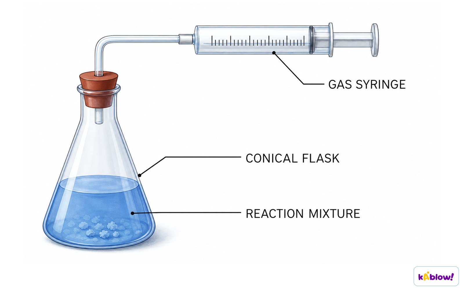
Monitor a gas-producing reaction
- A gas syringe can record gas volume against time. The reviewed apparatus connects a reaction flask to a freely moving syringe plunger.
- At controlled temperature and pressure, gas volume can act as a proxy for amount. A volume rate such as cm³ s⁻¹ is not yet a concentration rate in mol dm⁻³ s⁻¹.
- Check for leaks, mixing delay, syringe friction and sufficient collection capacity. A plateau indicates no further collected gas under the conditions, not necessarily that both reactants have been consumed.
Record gas volume over time
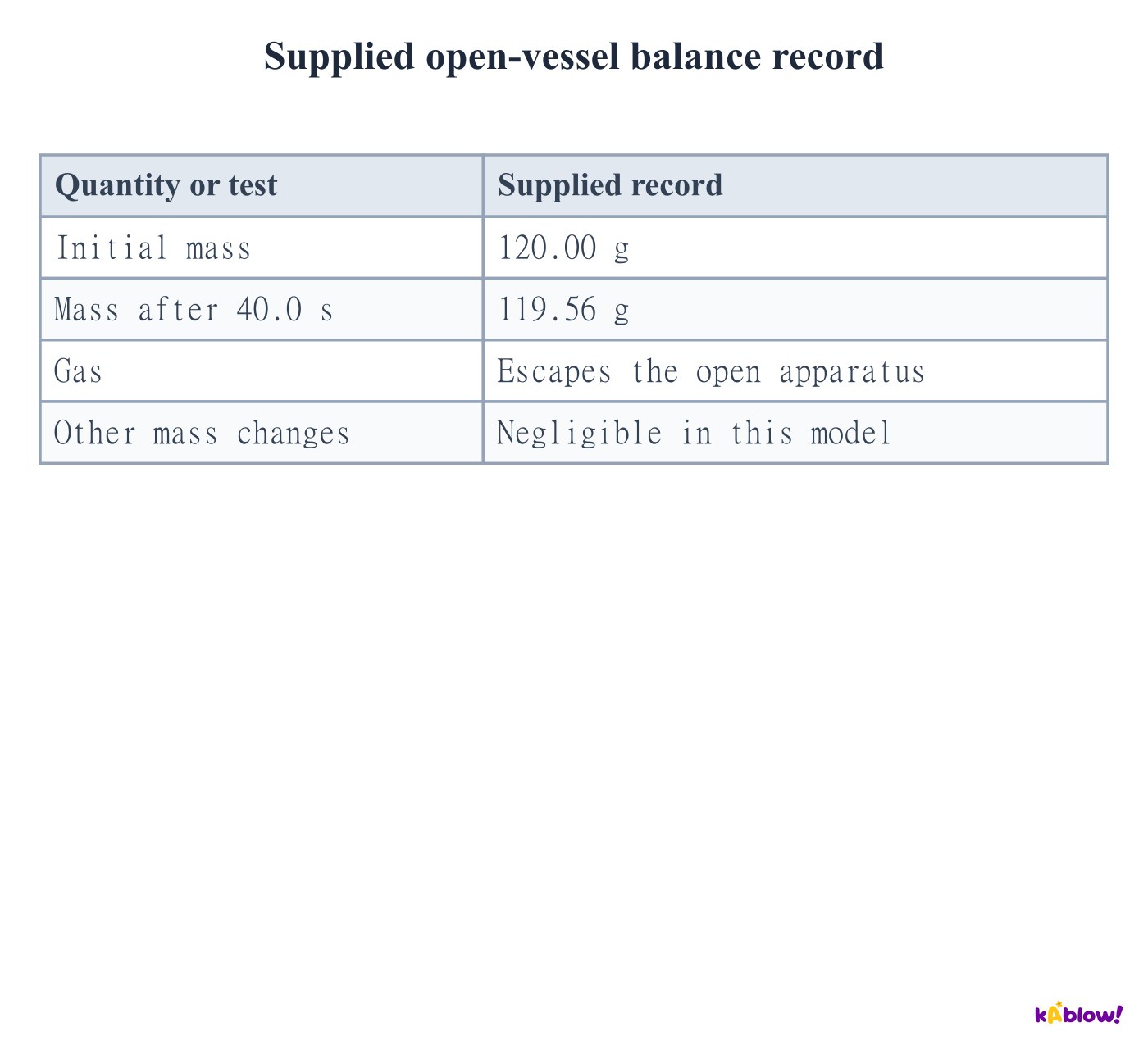
Use mass loss when gas escapes
- If a gas-producing reaction releases gas from an open apparatus, the measured mass can decrease. Mass loss per unit time can then monitor the process.
- The gas must be allowed to escape for this method. A sealed gas-collection system can retain the gas mass even while reaction continues.
- Evaporation, spray and draughts can also change a balance reading. Choose conditions that minimise these effects and keep the measured proxy distinct from a chemical concentration rate.
Supplied open-vessel balance record
Convert an optical measurement using calibration
- A colorimeter monitors light absorption by a suitable coloured species. Use a calibration or a justified proportionality to convert absorbance to concentration.
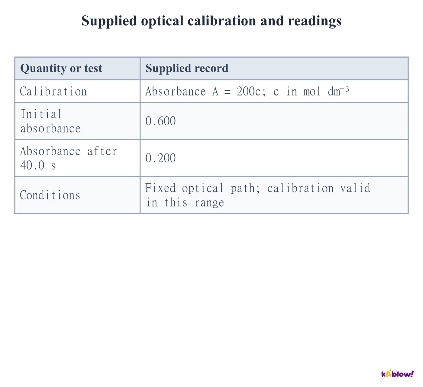
- In the supplied linear calibration, absorbance A = 200c for c in mol dm⁻³. The concentration falls from 0.00300 to 0.00100 mol dm⁻³ over 40.0 s.
- The average positive disappearance rate is therefore 0.00200/40.0 = 0.0000500 mol dm⁻³ s⁻¹. Absorbance change per second alone has different units.
Supplied optical calibration and readings
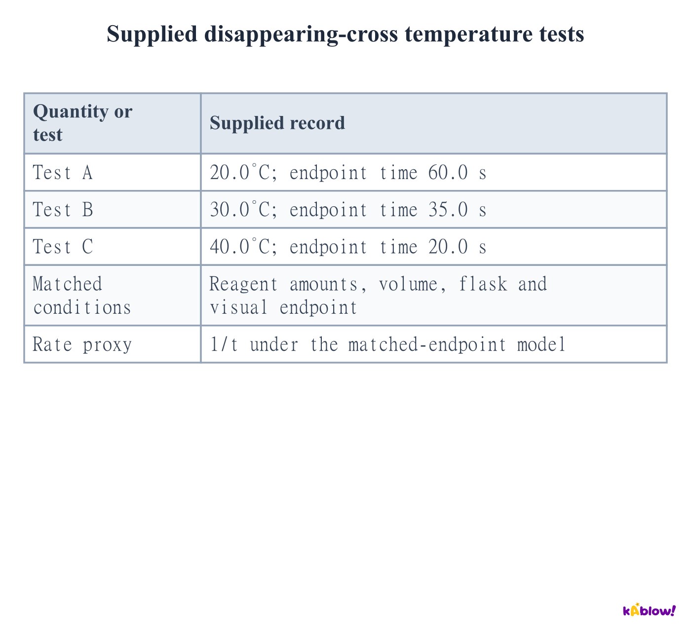
Interpret a fixed-endpoint timing method
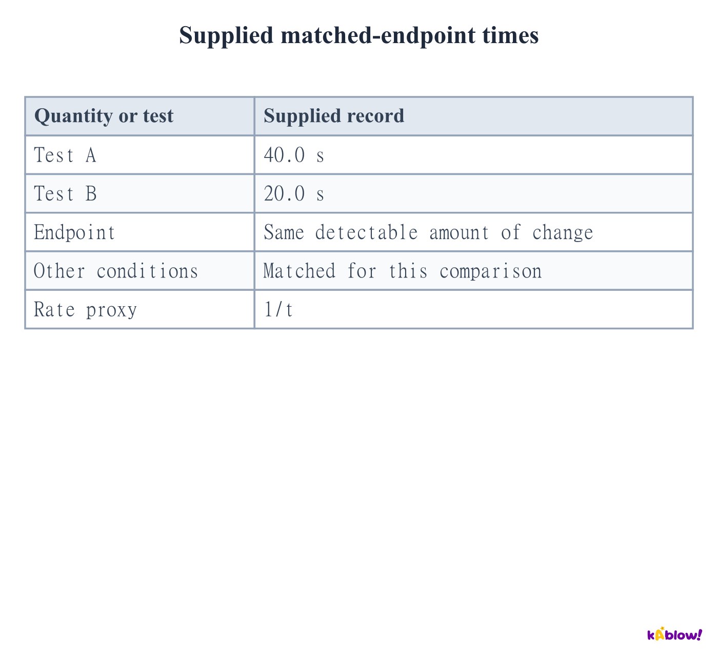
- When the same detectable change marks the endpoint in matched experiments, its completion time can be used to compare relative rates.
- The quantity 1/t is a rate proxy with units s⁻¹. It is not automatically a concentration rate unless the corresponding concentration change is known.
- Keep the endpoint, total volume and viewing conditions fixed. Different amounts of change at the endpoint can invalidate a simple inverse-time comparison.
Supplied matched-endpoint times
Read a Maxwell–Boltzmann energy distribution
- The curve describes the distribution of translational molecular energies in a classical gas at a specified temperature. The energy axis must not be confused with a speed axis.
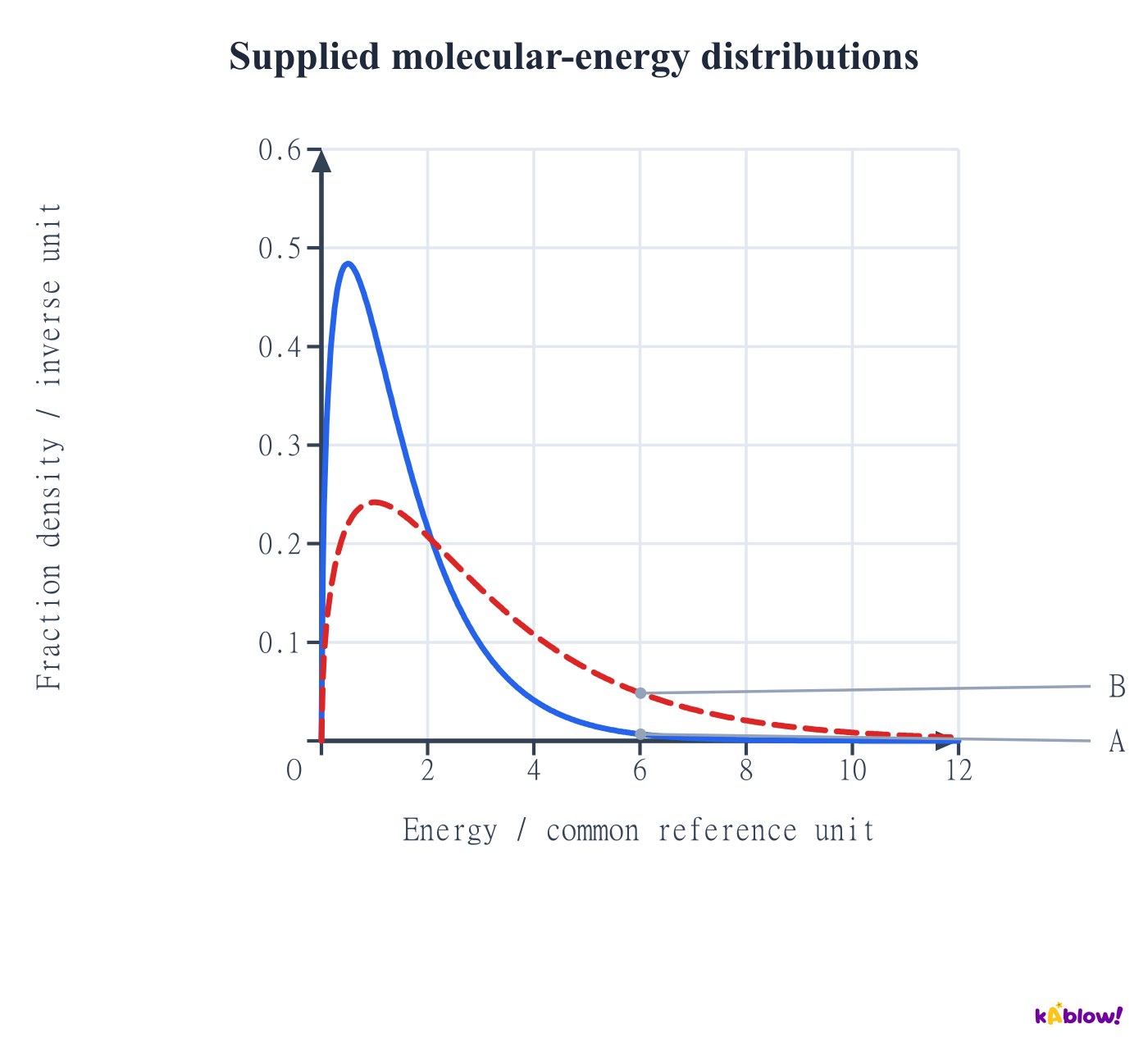
- For the normalised energy-density graph, the full area is one. The area over an energy interval gives the fraction of molecules in that interval; curve height alone is not that fraction.
- The energy density is zero at zero energy, rises to a maximum and approaches zero along a high-energy tail. The tail continues beyond the visible plot.
Supplied molecular-energy distributions
Explain the effect of increasing temperature
- For the same gas and fixed particle number, increasing temperature broadens the energy distribution and shifts its maximum towards higher energy, with a lower peak.
- A larger fraction exceeds a fixed positive activation-energy threshold. Increased particle speeds can also raise collision frequency; the larger high-energy fraction is central to the usual AQA explanation.
- Temperature describes the ensemble distribution. It does not require every individual molecule to gain an identical amount of energy, and a 10°C rise does not impose one universal rate factor.
Supplied molecular-energy distributions
Distinguish energy eligibility from successful collisions
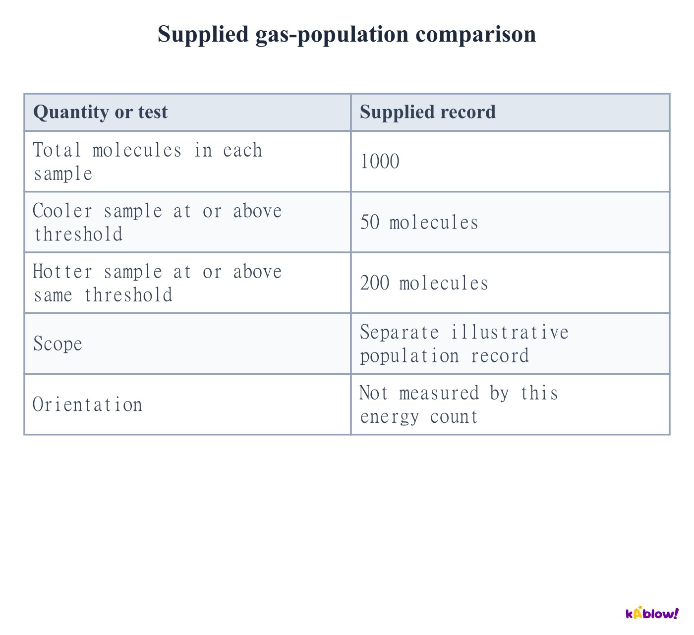
- Molecules above a threshold have sufficient energy in the simplified model, but suitable encounters and orientation are still required.
- Use a supplied population record to calculate fractions without claiming that every eligible molecule reacts immediately.
- At fixed temperature, an increased collision count does not by itself shift the normalised energy distribution. Keep population fractions separate from encounters per second.
Supplied gas-population comparison
Explain concentration effects without a universal rate law
- Concentration measures amount per volume of solution. At fixed temperature, more reacting particles per unit volume can increase collision frequency.
- This does not mean that increasing concentration increases the particles’ energy distribution or lowers the activation barrier.
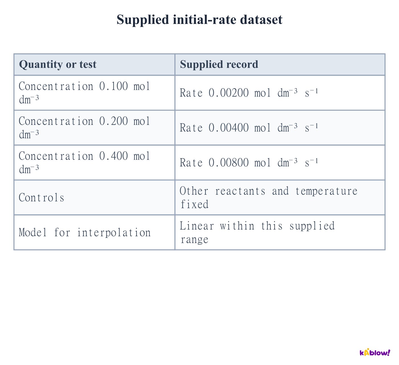
- The precise relationship between measured rate and concentration is empirical. Doubling a reactant concentration does not always double the rate; the supplied linear dataset supports that conclusion only for its stated range and conditions.
Supplied initial-rate dataset
Explain isothermal compression of reacting gases
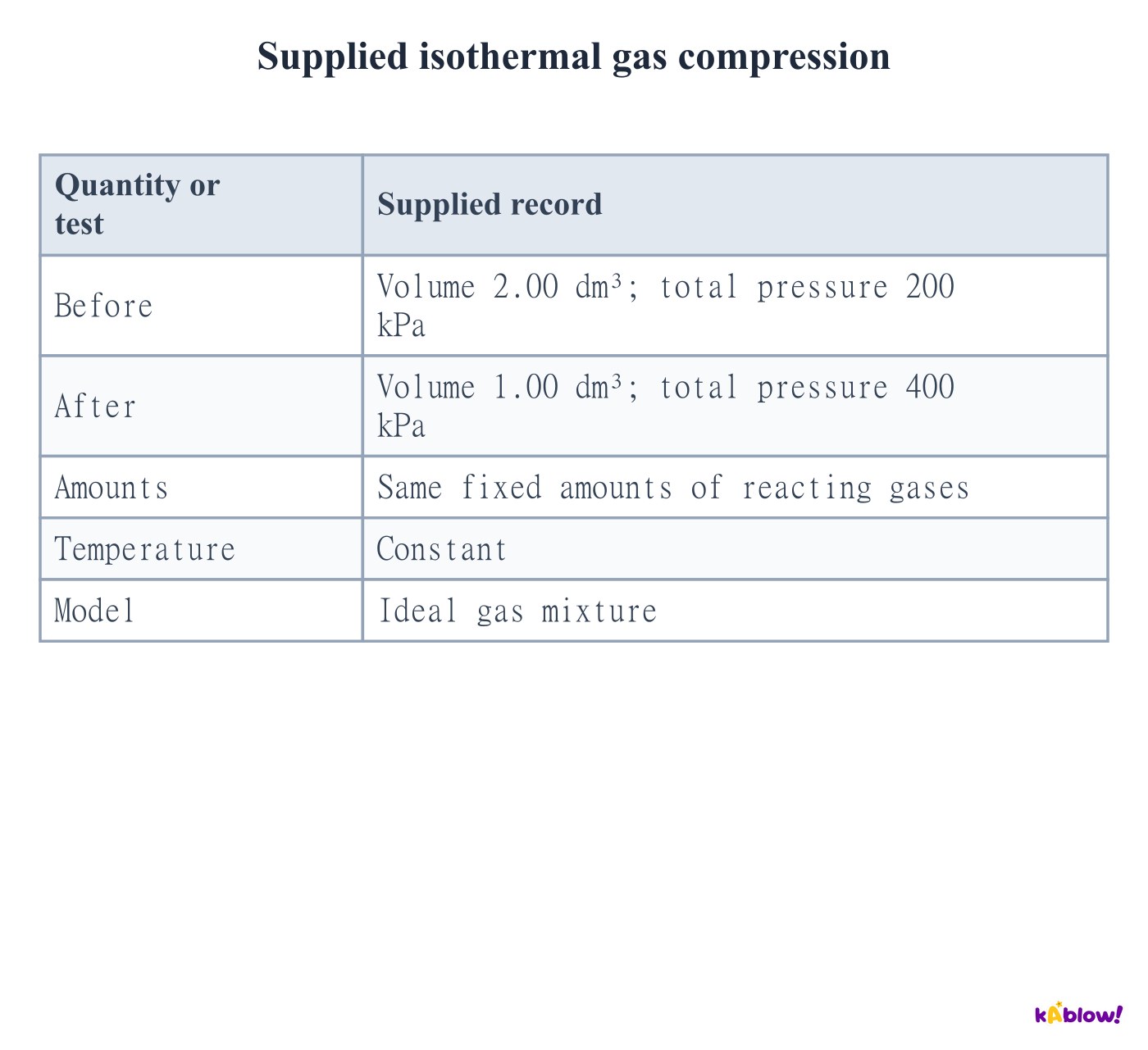
- Compressing a fixed gas sample at constant temperature reduces its volume and raises the relevant gas concentrations and partial pressures.
- More reacting particles per unit volume can increase collision frequency. The normalised energy distribution remains the same at fixed temperature in the ideal-gas model.
- A pressure change must be linked to how the system was changed. Temperature changes or adding an inert gas are not the same intervention as isothermal compression.
Supplied isothermal gas compression
Separate total pressure from reacting partial pressures
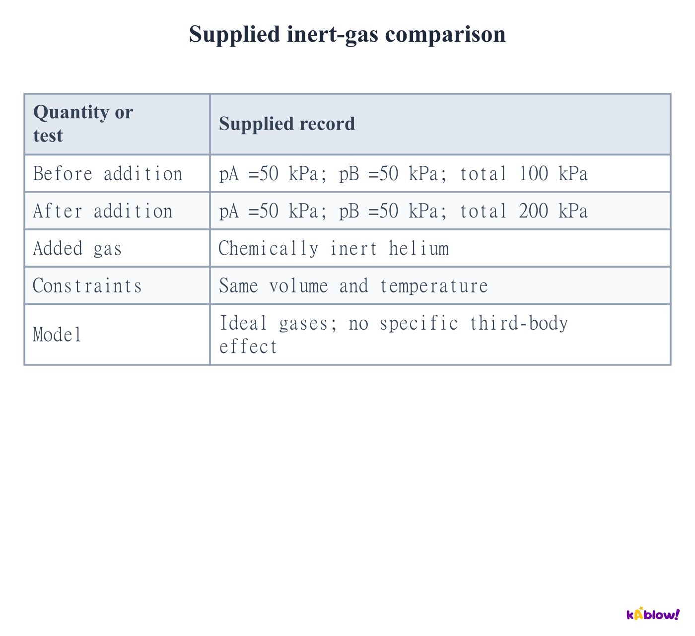
- Adding an inert gas at fixed volume and temperature raises total pressure without changing the amounts or concentrations of the reacting gases.
- In the stated ideal-gas collision model, unchanged reacting concentrations and temperature give no rate increase simply from the larger total pressure.
- Specify the constraint: adding inert gas at constant total pressure can instead expand the volume and change reacting concentrations.
Supplied inert-gas comparison
Relate surface area to heterogeneous reaction rate
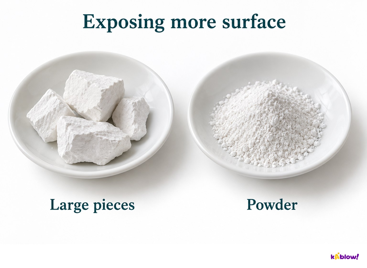
- Breaking the same mass of solid into smaller particles exposes more surface where contact with another phase can occur.
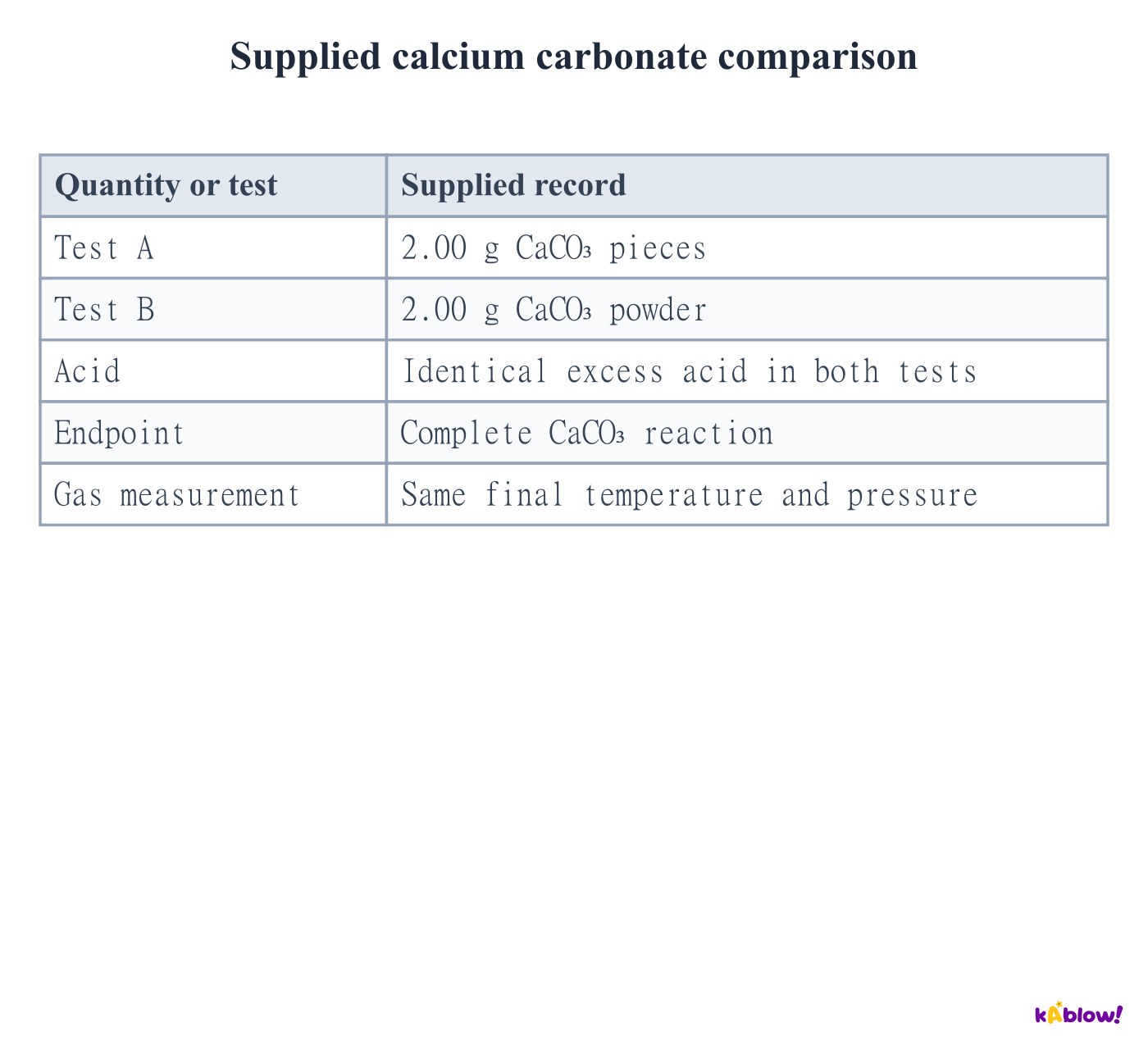
- The reviewed chalk comparison illustrates pieces and powder. With otherwise matched conditions, the powder can have a higher initial rate while the total reacting amount is unchanged.
- For equal solid amount reacting completely with excess acid, final gas amount can be the same despite different times. Surface area affects access to reaction sites, not the energy threshold by itself.
Expose more solid surface
Explain how a catalyst participates and is regenerated
- A catalyst increases reaction rate by providing an alternative route with a lower activation barrier. It can participate in individual steps and be regenerated overall.
- It does not have to remain uninvolved in every collision or appear unchanged in every intermediate. Real catalysts can also be deactivated or poisoned.
- The same reactant and product enthalpies mean the reaction enthalpy is unchanged. In the supplied profiles, compare barrier heights from the common starting level.
Supplied alternative pathway profiles
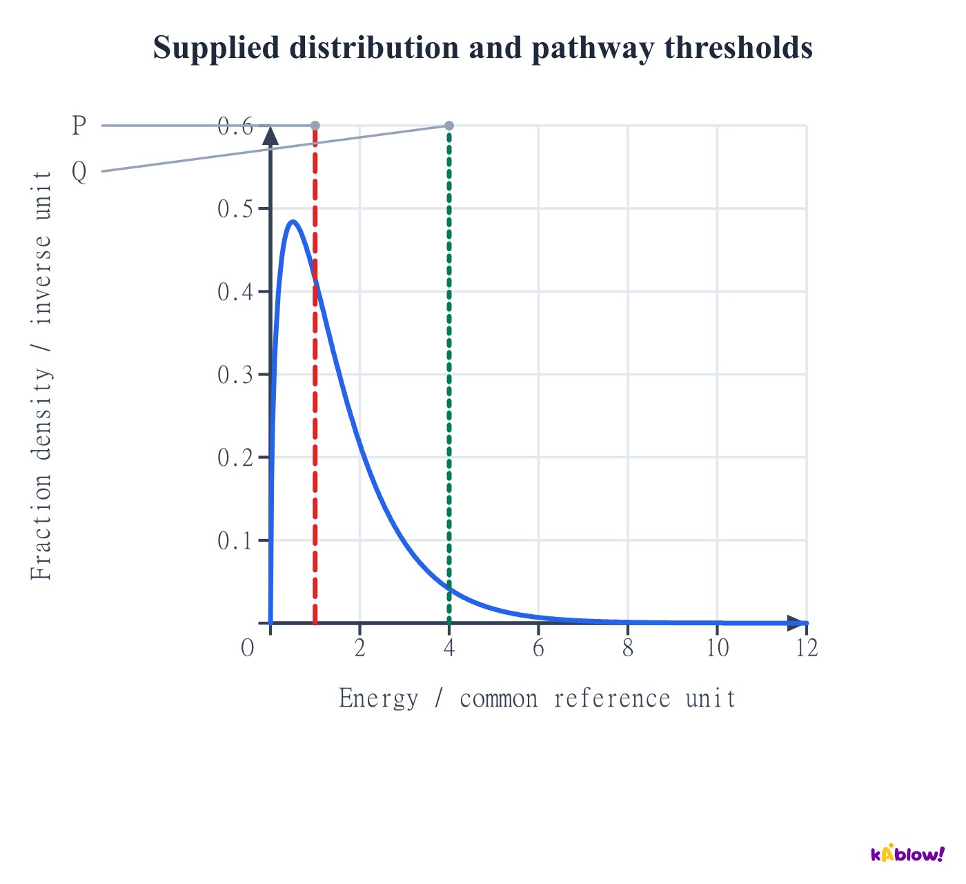
Show catalysis on an energy-distribution graph
- At fixed gas temperature, a catalyst does not shift the equilibrium molecular-energy distribution to higher energies.
- Instead, a lower pathway threshold makes a larger existing fraction energetically eligible. Compare the areas to the right of the two threshold lines on the same curve.
- This graph separates the energy distribution from the reaction pathway. Eligibility still does not guarantee that every individual encounter reacts.
Supplied distribution and pathway thresholds
Distinguish homogeneous and heterogeneous catalysis
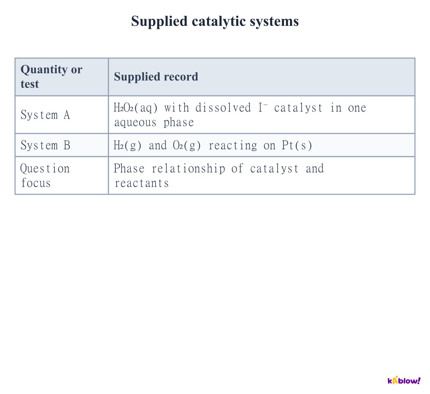
- A homogeneous catalyst is in the same phase as the reacting species. A heterogeneous catalyst is in a different phase, such as a solid surface used with gases.
- Phase means a physically distinct homogeneous region, not just a label such as liquid. Two immiscible liquids can be different phases despite sharing a physical state.
- The supplied examples separate an aqueous catalytic system from a gas–solid system. Mechanistic and adsorption details can be studied further in Transition Metals.
Supplied catalytic systems
Separate faster equilibration from equilibrium composition
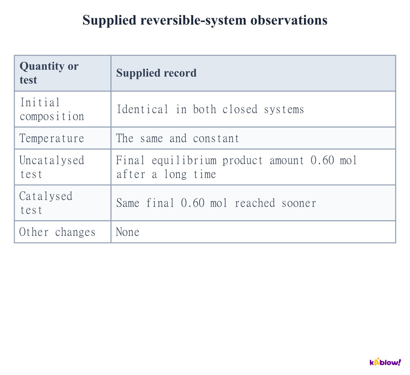
- For a reversible system at fixed temperature, a catalyst speeds the approach to equilibrium by facilitating both directions.
- It does not change the equilibrium constant or the final equilibrium composition for the same closed system and conditions.
- A larger amount observed after a short fixed time can reflect faster approach rather than a different final equilibrium yield. Keep time-limited observations separate from endpoint equilibrium measurements.
Supplied reversible-system observations
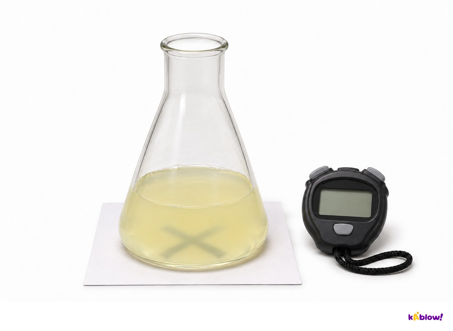
Investigate temperature using a disappearing-cross endpoint
- In the sodium thiosulfate–acid experiment, a sulfur suspension develops and obscures a cross viewed through the reaction mixture. Matched visual endpoints allow an inverse-time comparison.
- Equilibrate measured solutions to each target temperature, mix consistently and record the temperature and time. Keep reagent quantities, total volume, flask, liquid depth and viewing method consistent.
- The reaction can release sulfur dioxide. Use the teacher’s small-scale procedure with appropriate ventilation and eye protection, and avoid leaning over the open flask.
Time a disappearing-cross endpoint
Control variables and interpret the endpoint proxy
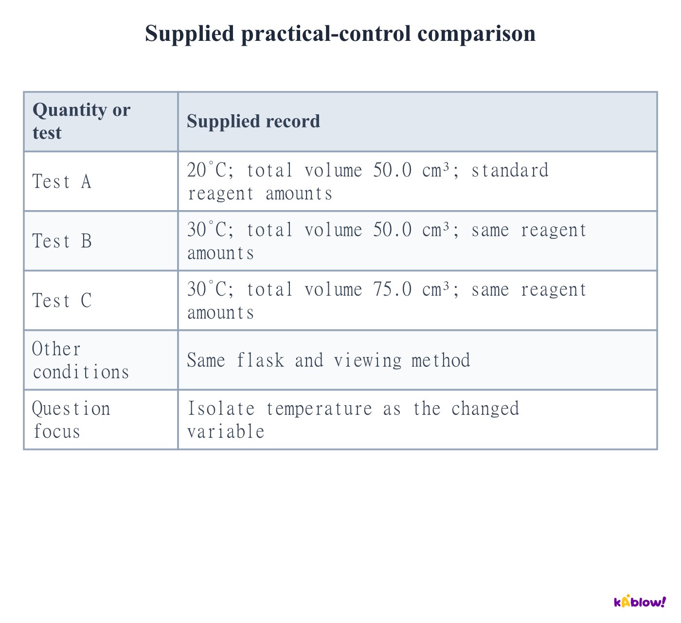
- To test temperature, change temperature while holding the other relevant conditions fixed. A different total liquid volume changes both concentrations and the optical path through the mixture.
- Use repeated tests and a consistent endpoint observer or objective optical measurement where possible. Mixing delay and timing can matter most for the fastest experiments.
- A 1/t comparison estimates relative rate only when approximately the same amount of visible change is needed each time. It does not independently determine a full rate equation.
Supplied practical-control comparison
Evaluate timing uncertainty and conclusions
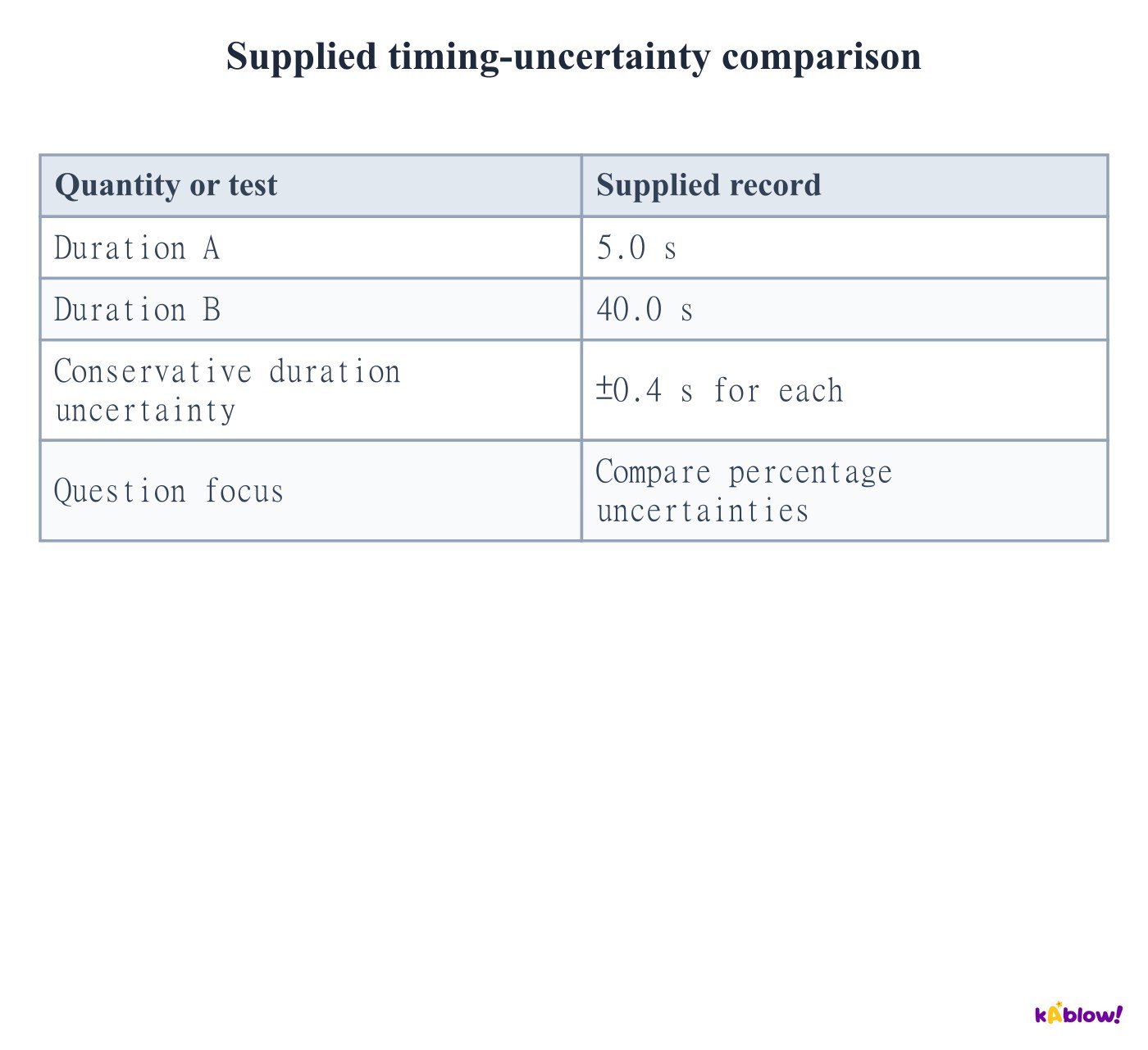
- For a duration obtained from two independently bounded time readings, a conservative absolute uncertainty can be estimated by adding the two reading uncertainties.
- The same absolute uncertainty gives a larger percentage uncertainty for a shorter time. Very rapid endpoints can therefore be difficult to compare precisely.
- Distinguish observations, model assumptions and conclusions. Repeat measurements can reveal spread, while systematic timing delay or a changing endpoint needs a method improvement.
Supplied timing-uncertainty comparison
슬라이드
연습 문제
무료 미리 보기 — 60개 중 8개 문제. 가입하면 전부 볼 수 있어요.
1.Which supplied collision meets both stated requirements?
Medium- AA only
- BB only
- CC only
- DA and B
2.What activation barrier belongs to the supplied lower-peak route Q?
Medium- A30 kJ mol⁻¹
- B40 kJ mol⁻¹
- C50 kJ mol⁻¹
- D90 kJ mol⁻¹
3.For the supplied reaction, what is the formation rate of B?
Medium- A0.010 mol dm⁻³ s⁻¹
- B0.020 mol dm⁻³ s⁻¹
- C0.040 mol dm⁻³ s⁻¹
- D0.080 mol dm⁻³ s⁻¹
4.What is the average product formation rate over the supplied 60.0 s interval?
Medium- A0.120 mol dm⁻³ s⁻¹
- B0.00720 mol dm⁻³ s⁻¹
- C0.00200 mol dm⁻³ s⁻¹
- D2.00 mol dm⁻³ s⁻¹
5.Where is the supplied product curve’s positive formation rate greatest?
Medium- ANear 0 s
- BNear 20 s
- CNear 40 s
- DNear 60 s
6.Which rate is the supplied initial tangent estimate?
Medium- A0.00300 mol dm⁻³ s⁻¹
- B0.00400 mol dm⁻³ s⁻¹
- C0.0600 mol dm⁻³ s⁻¹
- D0.0800 mol dm⁻³ s⁻¹
7.What average gas-volume rate follows between 10 and 20 s in the supplied collection record?
Medium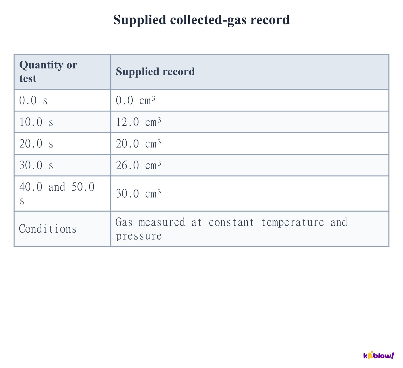
- A0.080 cm³ s⁻¹
- B0.800 cm³ s⁻¹
- C2.00 cm³ s⁻¹
- D8.00 cm³ s⁻¹
8.What average positive mass-loss rate follows from the supplied balance record?
Medium- A0.0110 g s⁻¹
- B0.440 g s⁻¹
- C1.10 g s⁻¹
- D−0.0110 g s⁻¹
기출 문제
이 주제의 기출 문제 연습이 곧 나와요.
곧 출시