Rate Equations

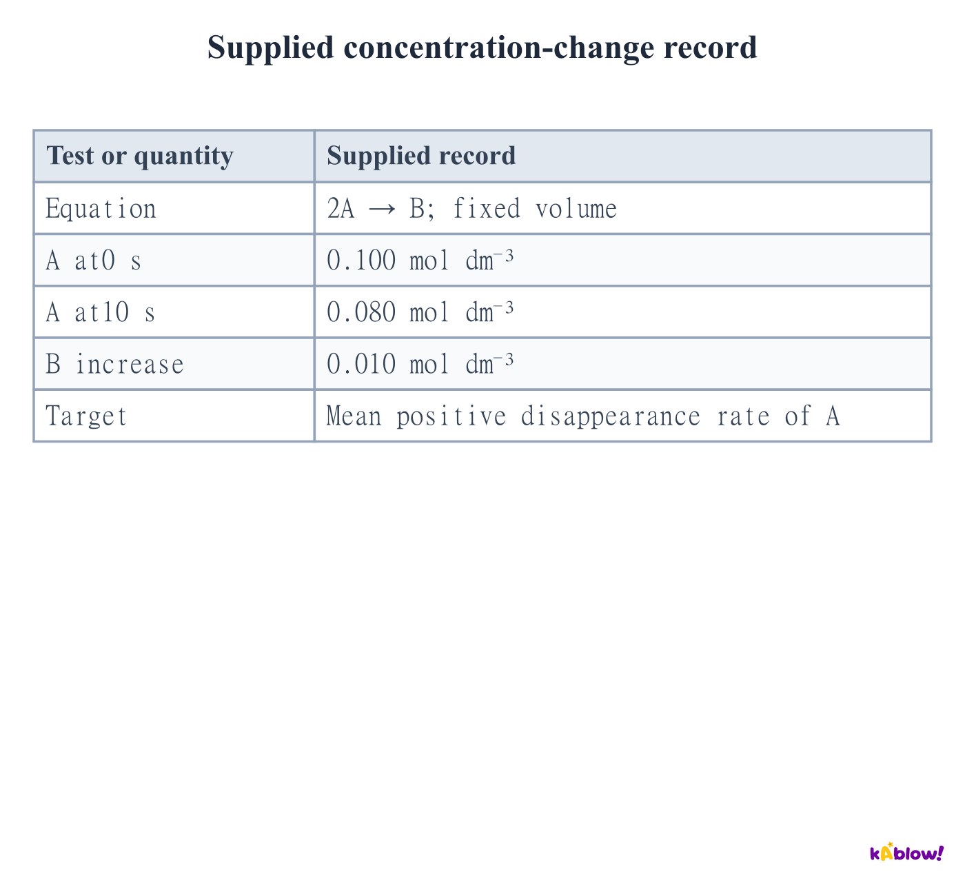
## State which rate you are measuring - A species disappearance rate is −Δ[A]/Δt and is positive when A decreases. A formation rate is +Δ[B]/Δt. State concentration and time units. - For 2A→B at constant volume, disappearance of A is twice formation of B. The coefficient-normalised reaction rate is −½d[A]/dt=d[B]/dt. - The supplied finite interval gives a mean rate. An instantaneous rate is obtained from a tangent at the chosen time. 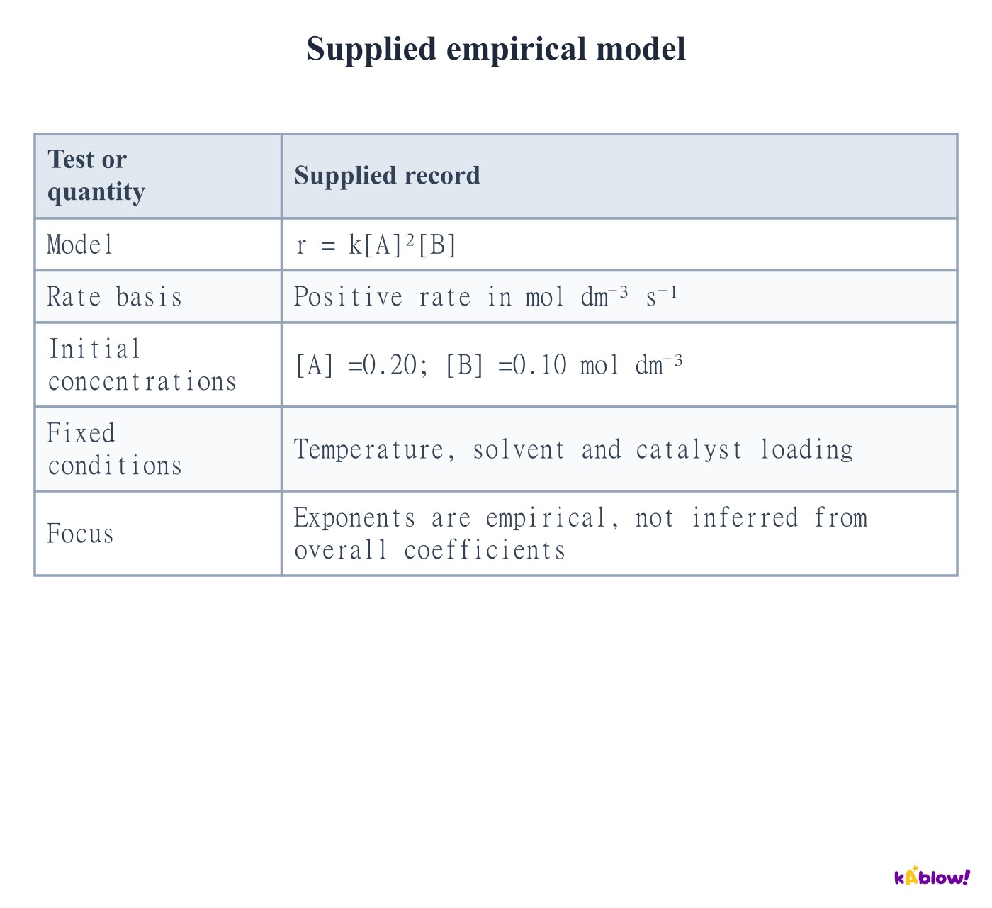## Read an empirical rate equation - In r=k[A]^m[B]^n, m and n are orders with respect to A and B. Overall order is m+n. Determine these exponents experimentally. - The rate equation does not usually follow directly from overall reaction coefficients. AQA examples emphasise zero, first and second orders; other values occur in chemistry. - For r=k[A]²[B], doubling A alone multiplies rate by four, while doubling B alone multiplies it by two. Use the same defined rate basis throughout. 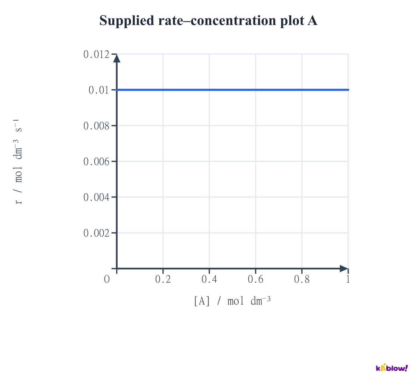## Recognise zero order from rate versus concentration - A horizontal positive rate–concentration line shows that changing the plotted concentration does not change rate over the investigated range. - The exponent for this species is zero: [A]⁰=1. This does not mean that A is absent from the overall chemical change. - The model has a finite range. It cannot describe continued consumption after the reactant has run out. 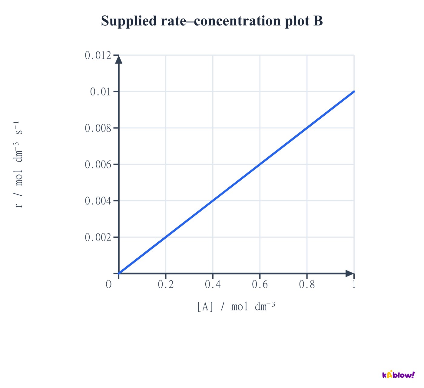## Recognise first order from rate versus concentration - A straight line through the origin on rate against concentration gives r proportional to[A] when other relevant concentrations and conditions are fixed. - Doubling[A] doubles rate. The gradient equals the appropriate constant only after accounting for any other fixed concentration factors. - Do not confuse this with concentration against time: a first-order concentration–time curve is exponential, not a straight line. 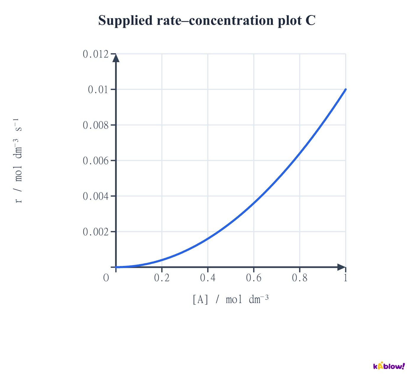## Recognise second order from rate versus concentration - For r=k[A]² with fixed conditions, rate against[A] is a quadratic curve through the origin. Doubling concentration multiplies rate by four. - A plot of r against[A]² would be linear through the origin for this model. - Always inspect both axes. A curved concentration–time trace alone does not establish second order merely because it looks steep. 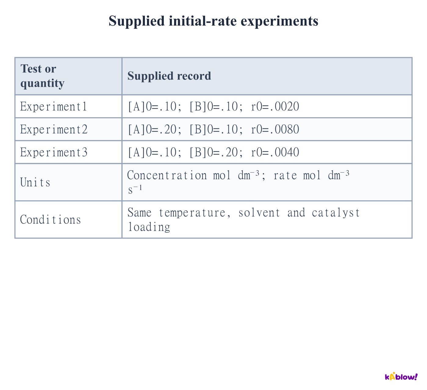## Use controlled initial-rate comparisons - Compare experiments1 and2: B is fixed while A doubles and rate quadruples. The order in A is two. - Compare experiments1 and3: A is fixed while B doubles and rate doubles. The order in B is one, giving r=k[A]²[B]. - Temperature, solvent, total-volume effects and catalyst loading must be controlled. Initial concentrations refer to the mixed reaction solution. 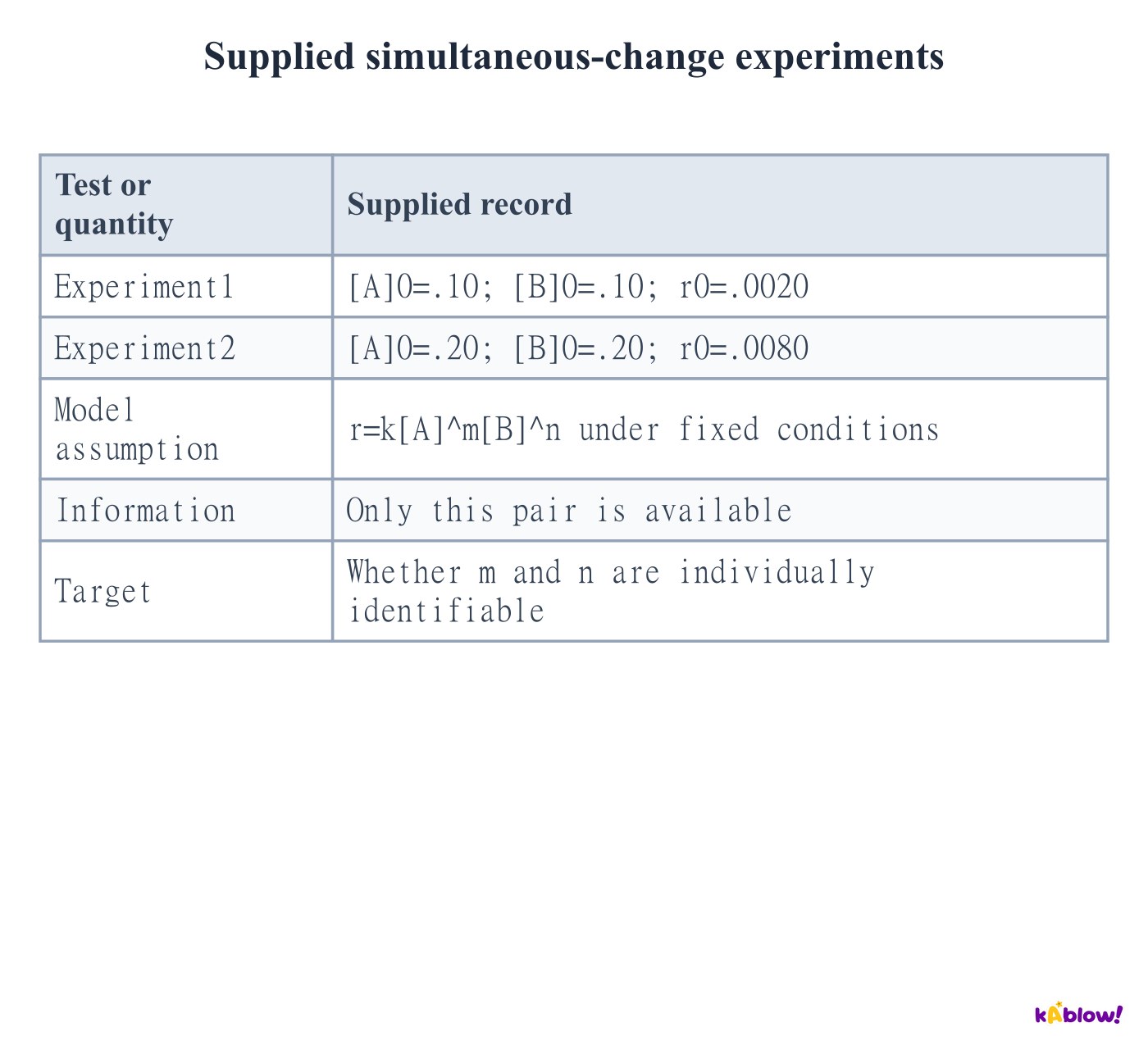## Identify when data cannot separate orders - If A and B both double and rate quadruples, the ratio equation is4=2^m×2^n. It constrains m+n=2. - This pair alone cannot distinguish m=2,n=0 from m=1,n=1 or m=0,n=2. - Simultaneous changes can still be analysed when enough independent experiments are supplied. Seek independent constraints rather than assuming every pair must change only one factor. 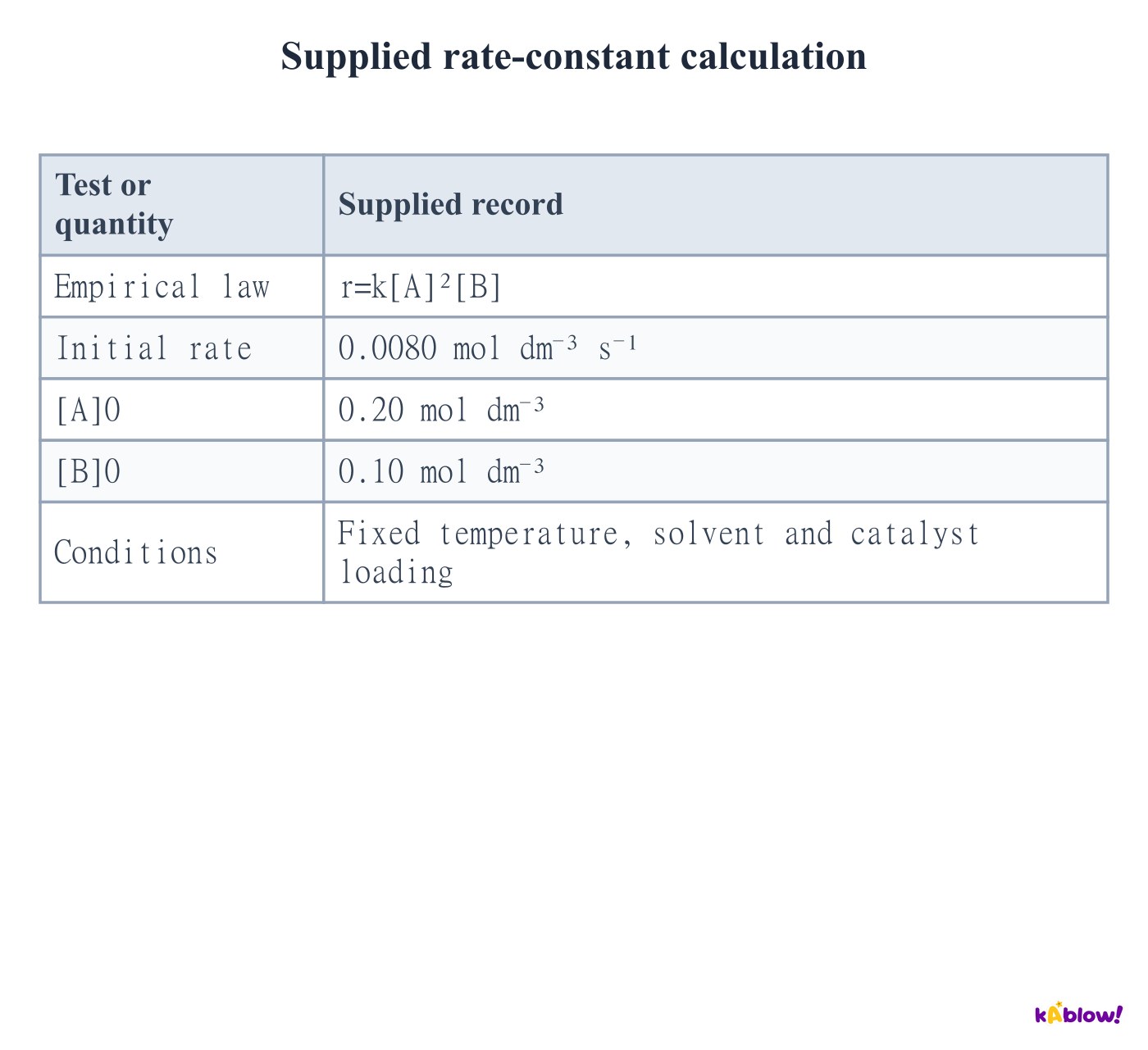## Calculate k after determining the orders - Rearrange r=k[A]²[B] to k=r/([A]²[B]). Substitute mixed concentrations with consistent units. - The supplied values give k=0.0080/(0.20²×0.10)=2.0 dm⁶ mol⁻² s⁻¹. - Changing concentrations alone does not change k under the stated fixed conditions. Temperature, reaction medium or catalyst changes can change its measured value. 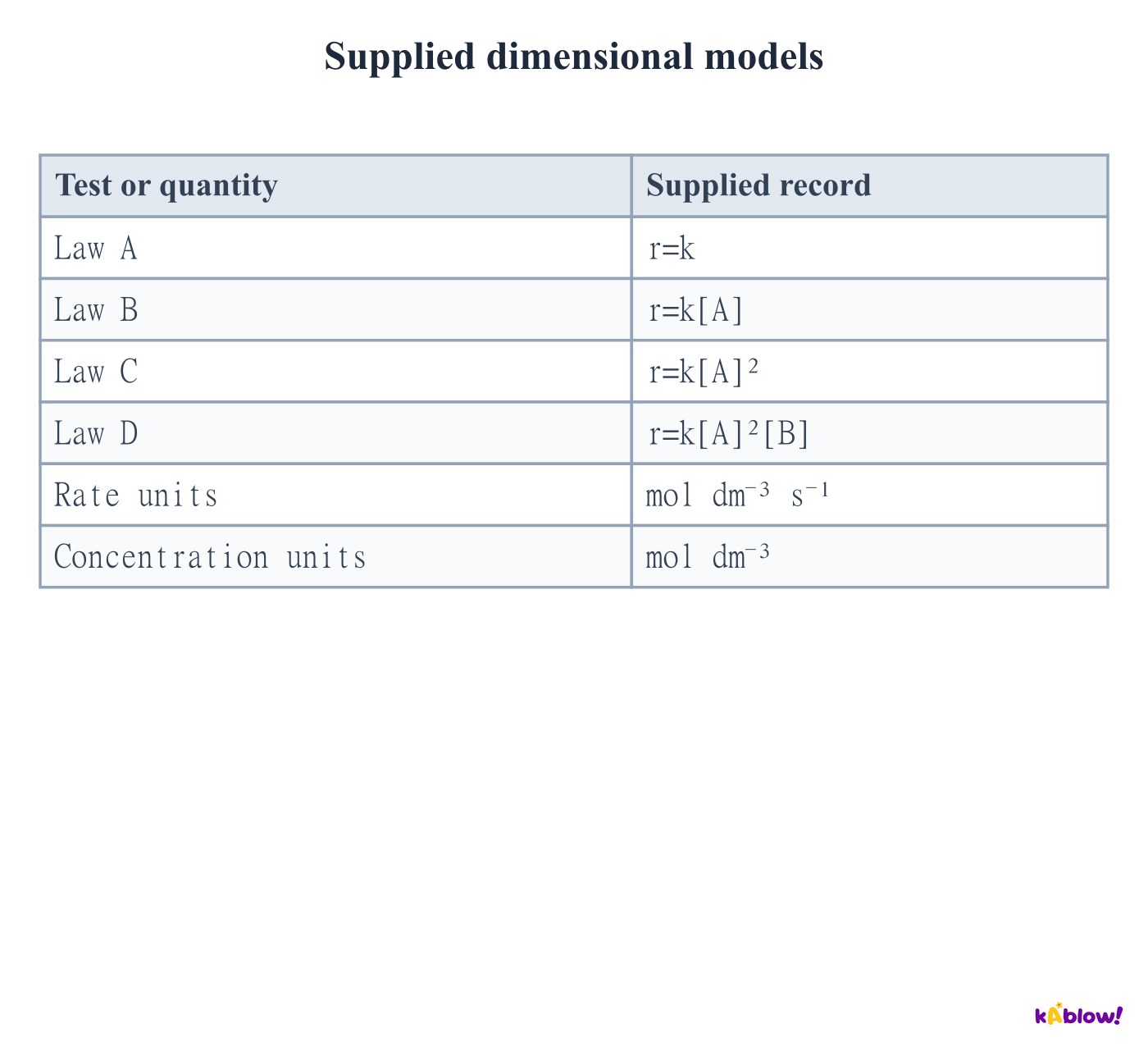## Derive rate-constant units - Divide rate units by concentration units raised to the overall order. For order n, units are(concentration)^(1−n) time⁻¹. - Zero-order k has mol dm⁻³ s⁻¹; first-order k has s⁻¹; second-order k has dm³ mol⁻¹ s⁻¹. - Third-order k has dm⁶ mol⁻² s⁻¹. Numerical values change if different concentration or time units are used, so record units with k. 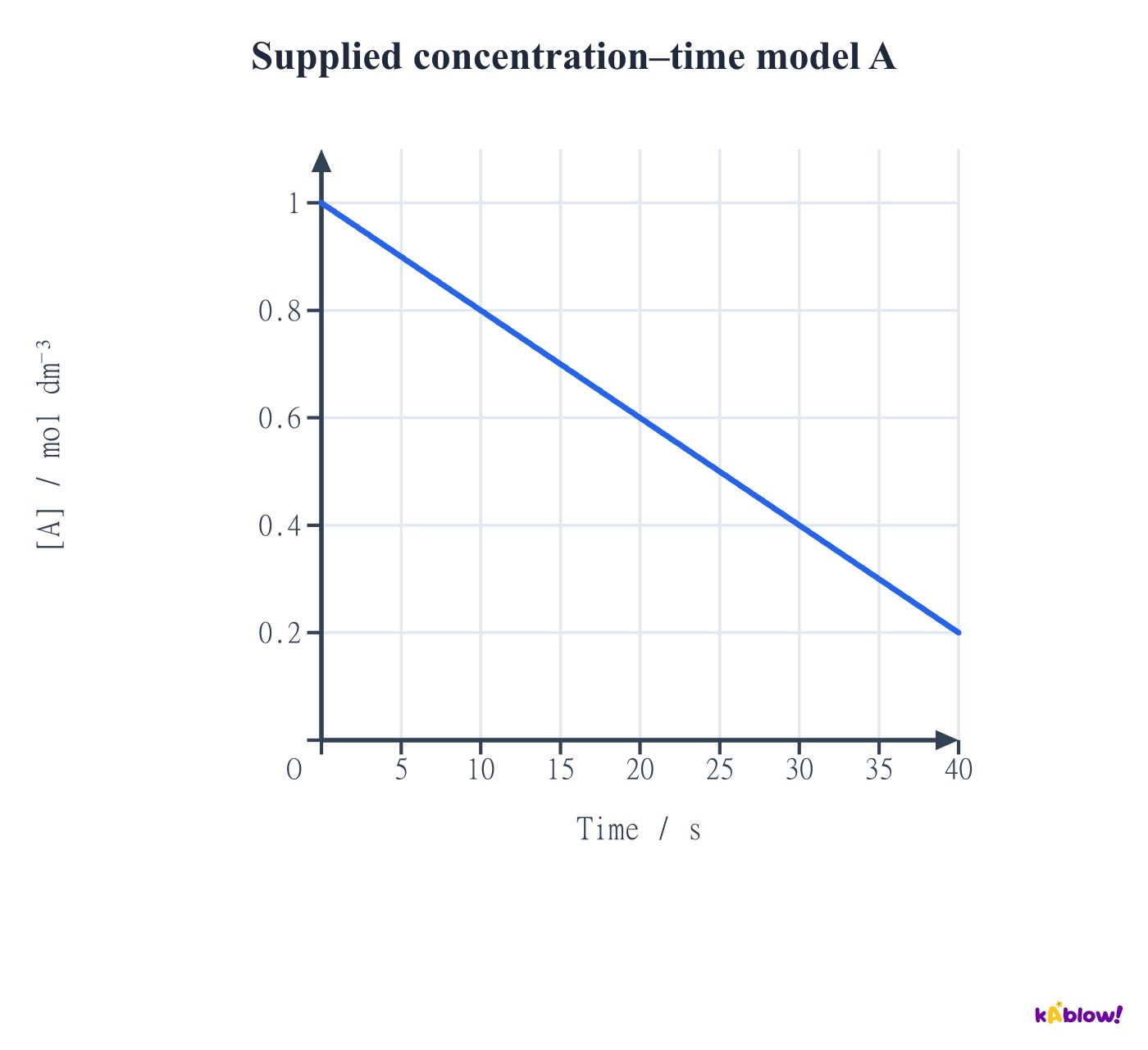## Read a linear concentration–time model - For the simple disappearance law−d[A]/dt=k, concentration is[A]0−kt while reactant remains. The graph has constant negative gradient. - Here[A]0=1.0 mol dm⁻³ and k=0.020 mol dm⁻³ s⁻¹. At40 s the concentration is0.20 mol dm⁻³. - The model predicts depletion at50 s. It must not be extended to negative concentrations, and it is linear rather than inverse proportionality. 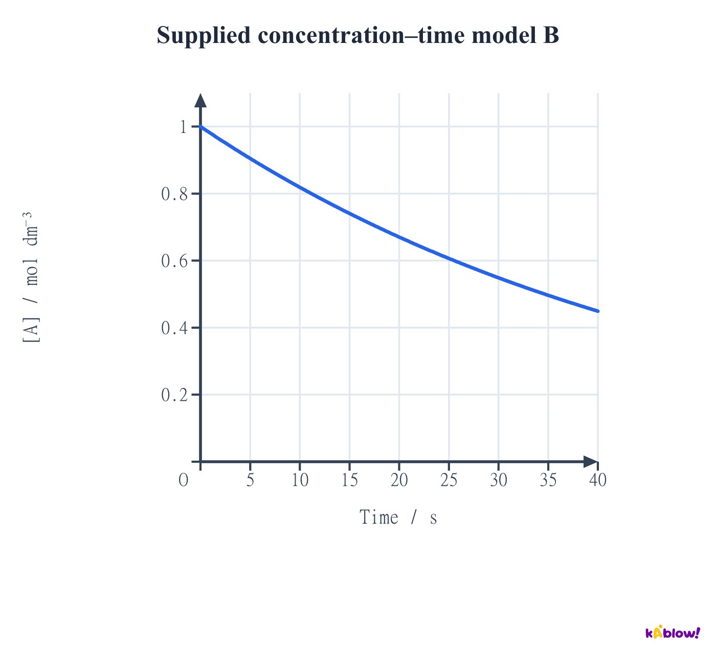## Read an exponential concentration–time model - For−d[A]/dt=k[A], the simple one-reactant model gives[A]=[A]0 exp(−kt). The negative gradient becomes smaller in magnitude as A decreases. - The supplied curve uses k=0.020 s⁻¹ and[A]0=1.0 mol dm⁻³. Its initial disappearance rate is0.020 mol dm⁻³ s⁻¹. - Extension: successive concentration halvings take equal times in this model, t½=ln2/k. This is a model-specific diagnostic, not a universal property of reactions. 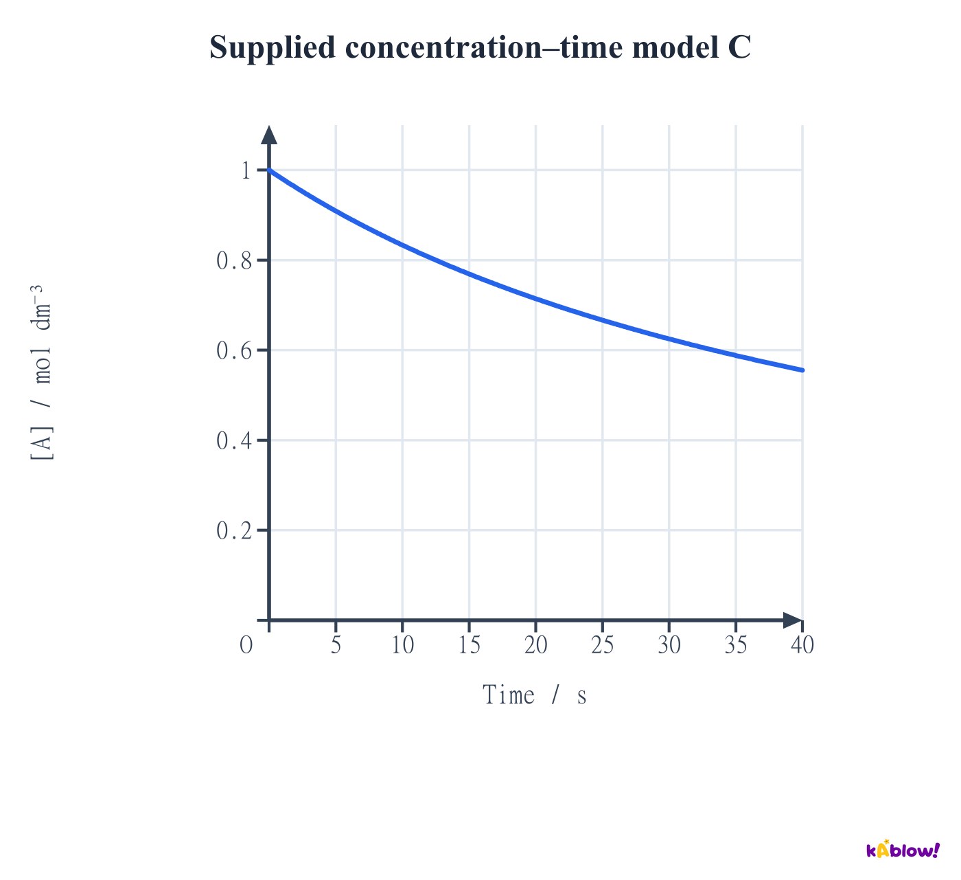## Compare concentration–time models fairly - The simple second-order model−d[A]/dt=k[A]² gives[A]=[A]0/(1+k[A]0t). Here k=0.020 dm³ mol⁻¹ s⁻¹ and[A]0=1.0 mol dm⁻³. - The supplied three time models share the same initial concentration and initial disappearance rate, while k has different units in each. - Do not identify order from absolute steepness: initial concentrations, k and plot scales affect it. Use quantitative model tests or controlled rate–concentration data. 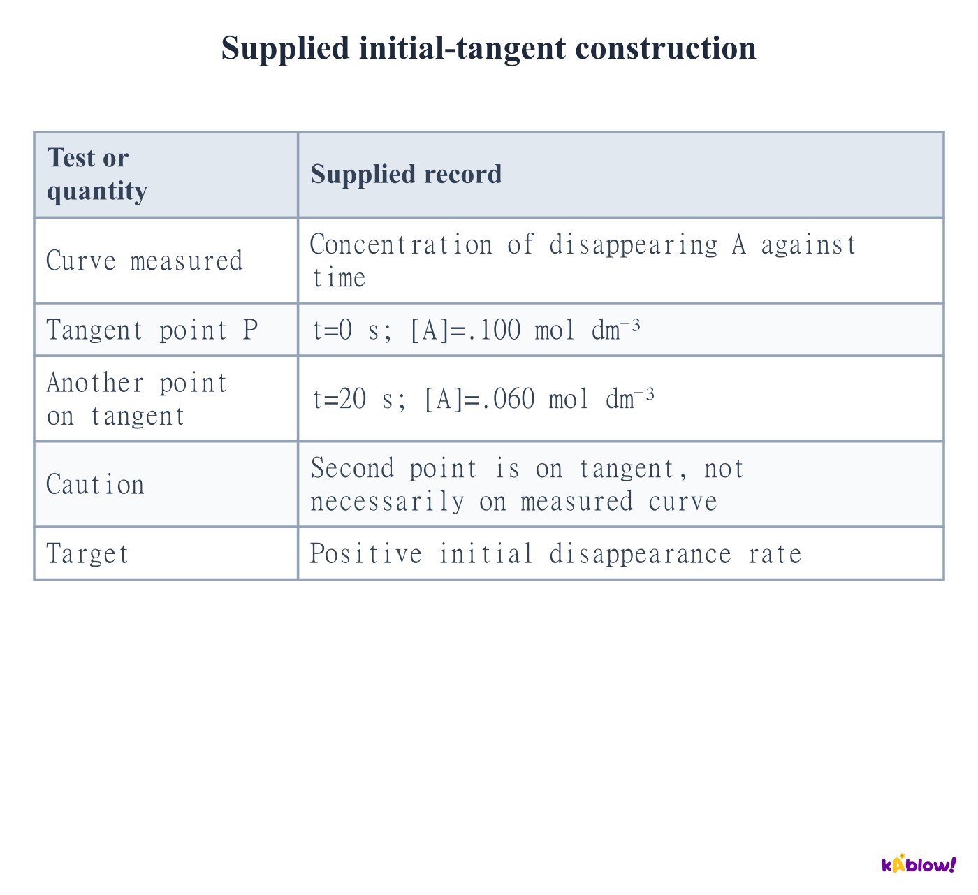## Find an initial rate from a tangent - Draw a tangent to the measured concentration–time curve at t=0. Use widely separated readable points on that tangent to estimate its gradient. - The supplied tangent slope is(0.060−0.100)/(20−0)=−0.0020 mol dm⁻³ s⁻¹, so the positive disappearance rate is0.0020 mol dm⁻³ s⁻¹. - A secant over a finite reaction interval gives an average rate. Mixing delay and early measurement uncertainty affect an initial tangent estimate. 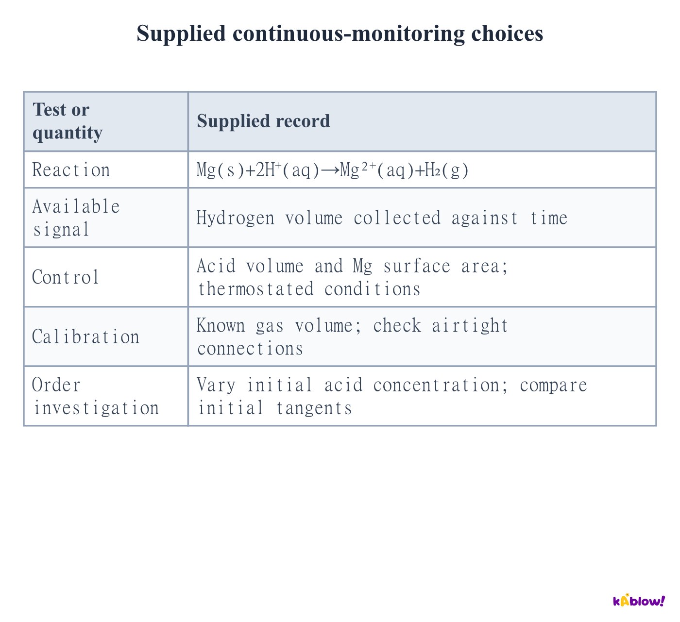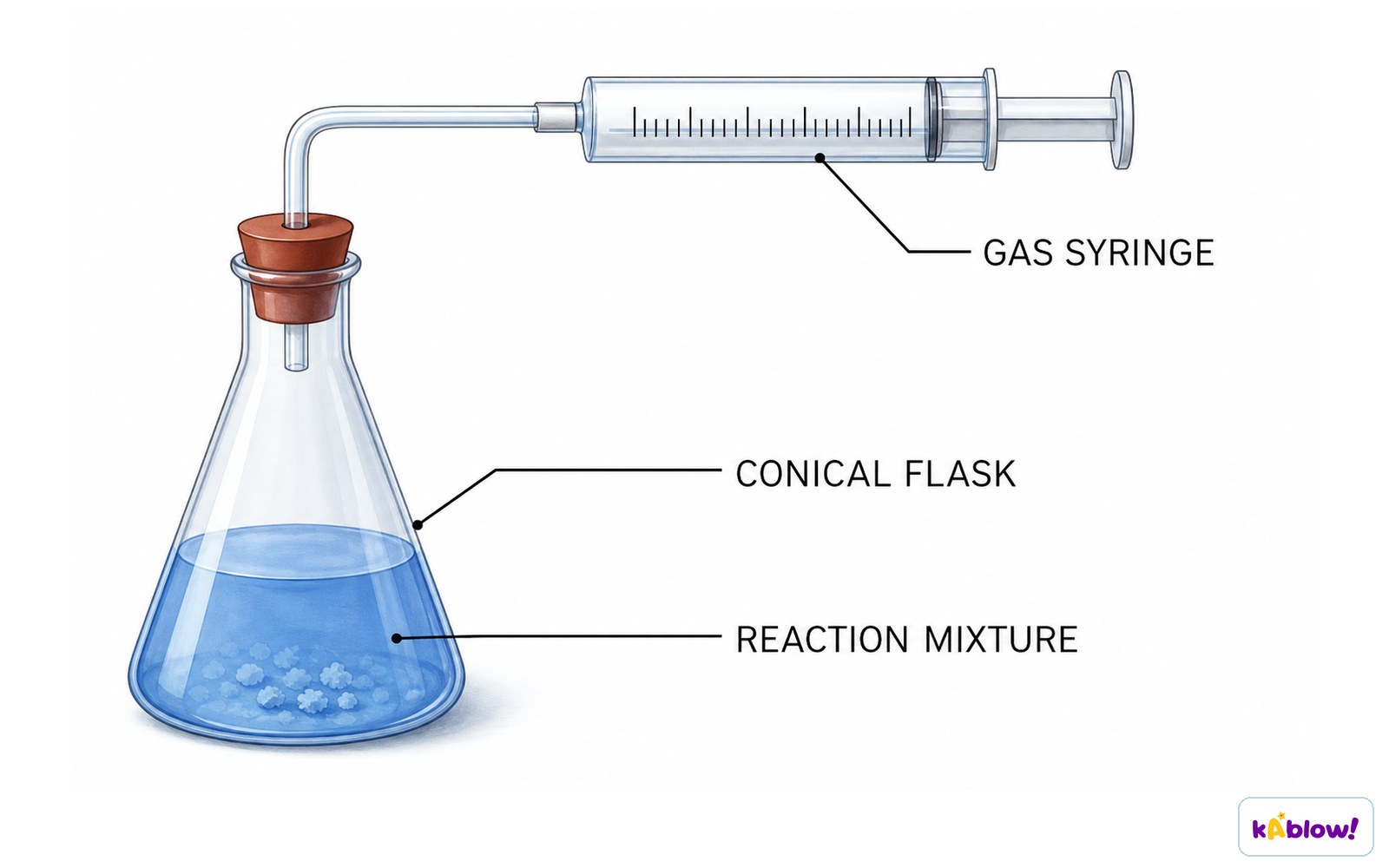## Plan continuous monitoring for required practical7 - Choose a signal that tracks reaction progress, such as gas volume, mass loss, colour or concentration. Relate signal change to the species or reaction rate being reported. - For Mg and acid, an airtight gas syringe can monitor hydrogen formation. Compare initial tangents across measured initial acid concentrations. - Keep magnesium surface area, acid volume and temperature controlled. Check gas leaks, syringe friction, mixing and timing; follow the practical risk assessment for acid and flammable hydrogen. 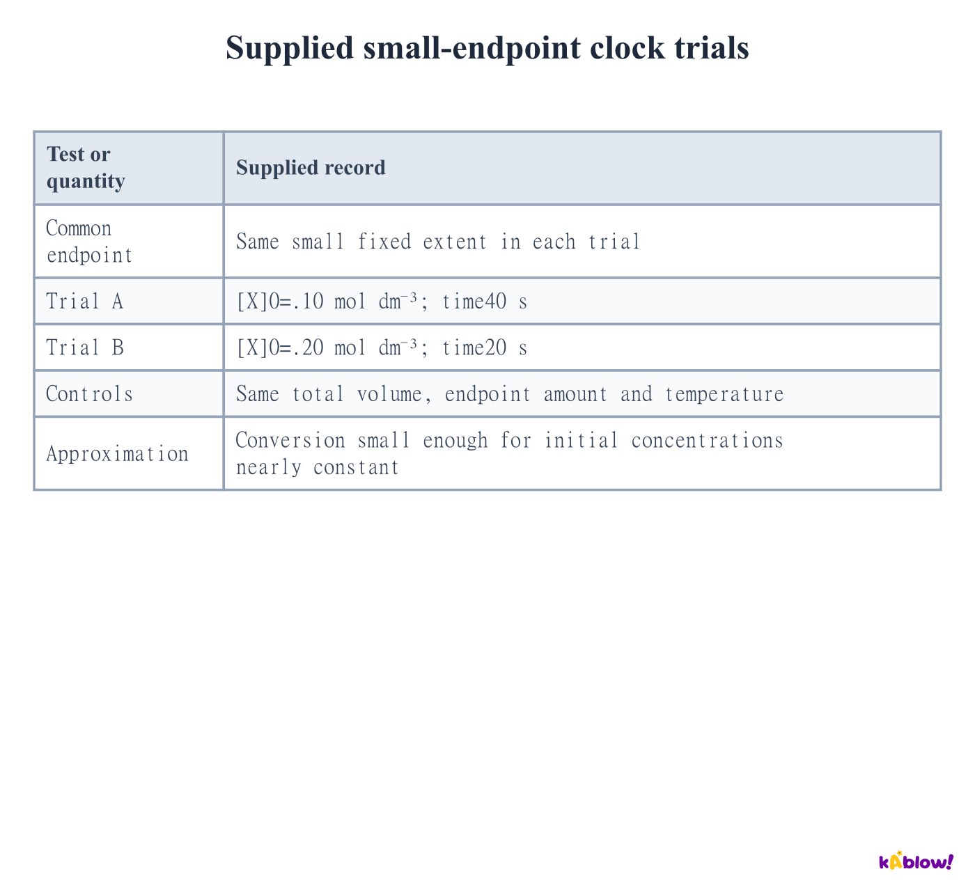## Use a small fixed clock endpoint - A clock measures the time to a known small extent. With the same endpoint amount and total volume, rate is approximately proportional to1/t when initial concentrations change little. - The supplied doubling of X halves time, so its initial-rate proxy doubles. This supports first order in X under the stated approximation and controls. - 1/t has units s⁻¹ and is a proxy, not automatically a concentration rate. Multiply the known endpoint concentration change by1/t when an absolute rate is required. 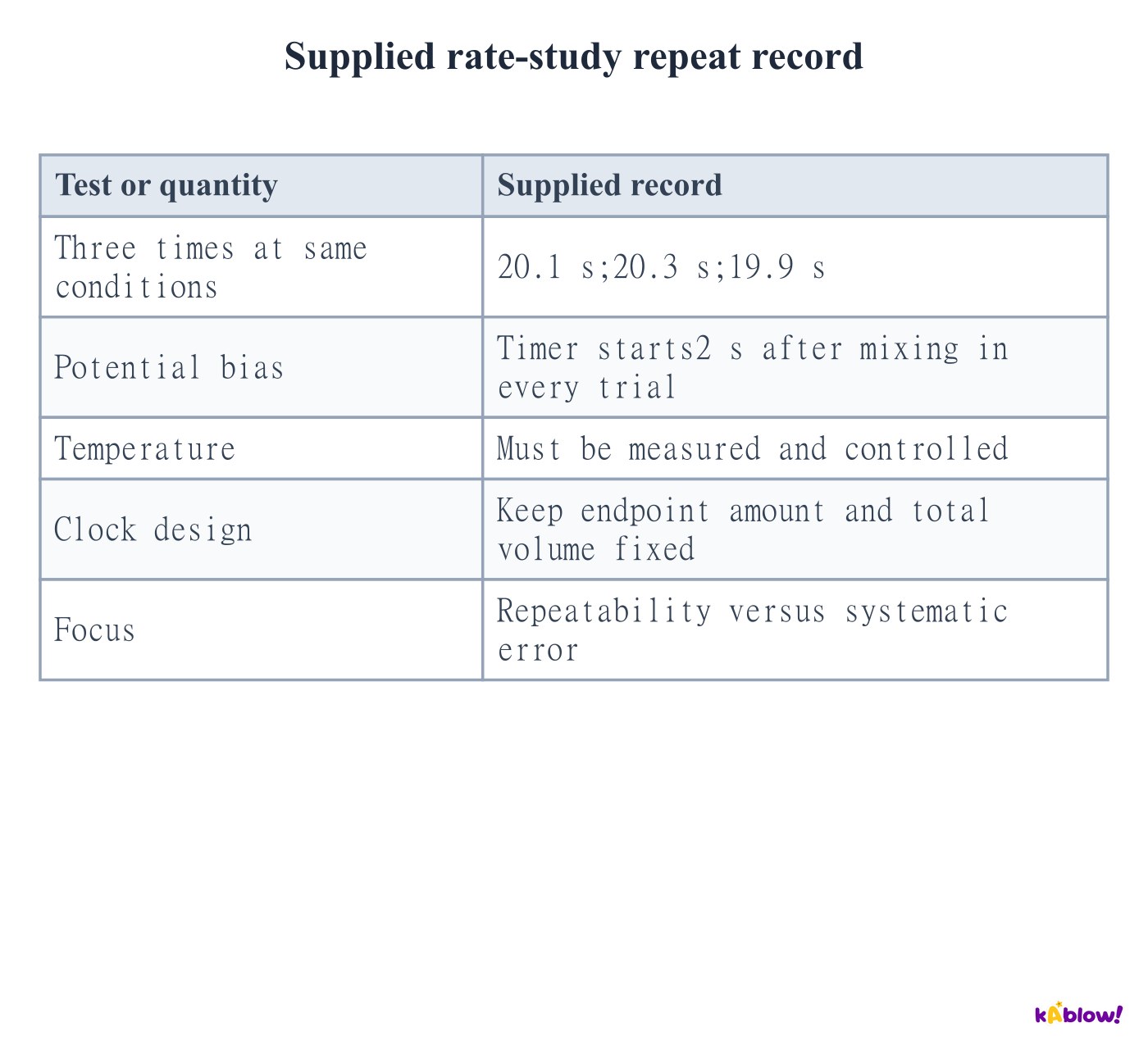## Separate repeatability from accuracy - Closely agreeing repeat times indicate repeatability. A common mixing or timing delay can still bias every result. - Repeat experiments, identify anomalous trials, calculate a justified mean and report measurement uncertainty. Do not assume a mean removes systematic error. - Control temperature, mixed volumes and endpoint amount. Use the same timing convention and improve rapid mixing or automatic detection where appropriate. 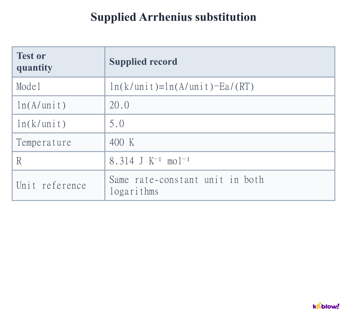## Use the Arrhenius equation with consistent units - Use k=A exp(−Ea/RT), or ln(k/unit)=ln(A/unit)−Ea/(RT). A and k have the same units; both logarithms use the same reference unit. - Use thermodynamic temperature in kelvin. With R=8.314 J K⁻¹ mol⁻¹, Ea must be in J mol⁻¹ before conversion to kJ mol⁻¹. - The supplied difference20−5=15 gives Ea=15×8.314×400=49884 J mol⁻¹, or49.9 kJ mol⁻¹ to three significant figures. The model assumes A and Ea apply over its investigated range. 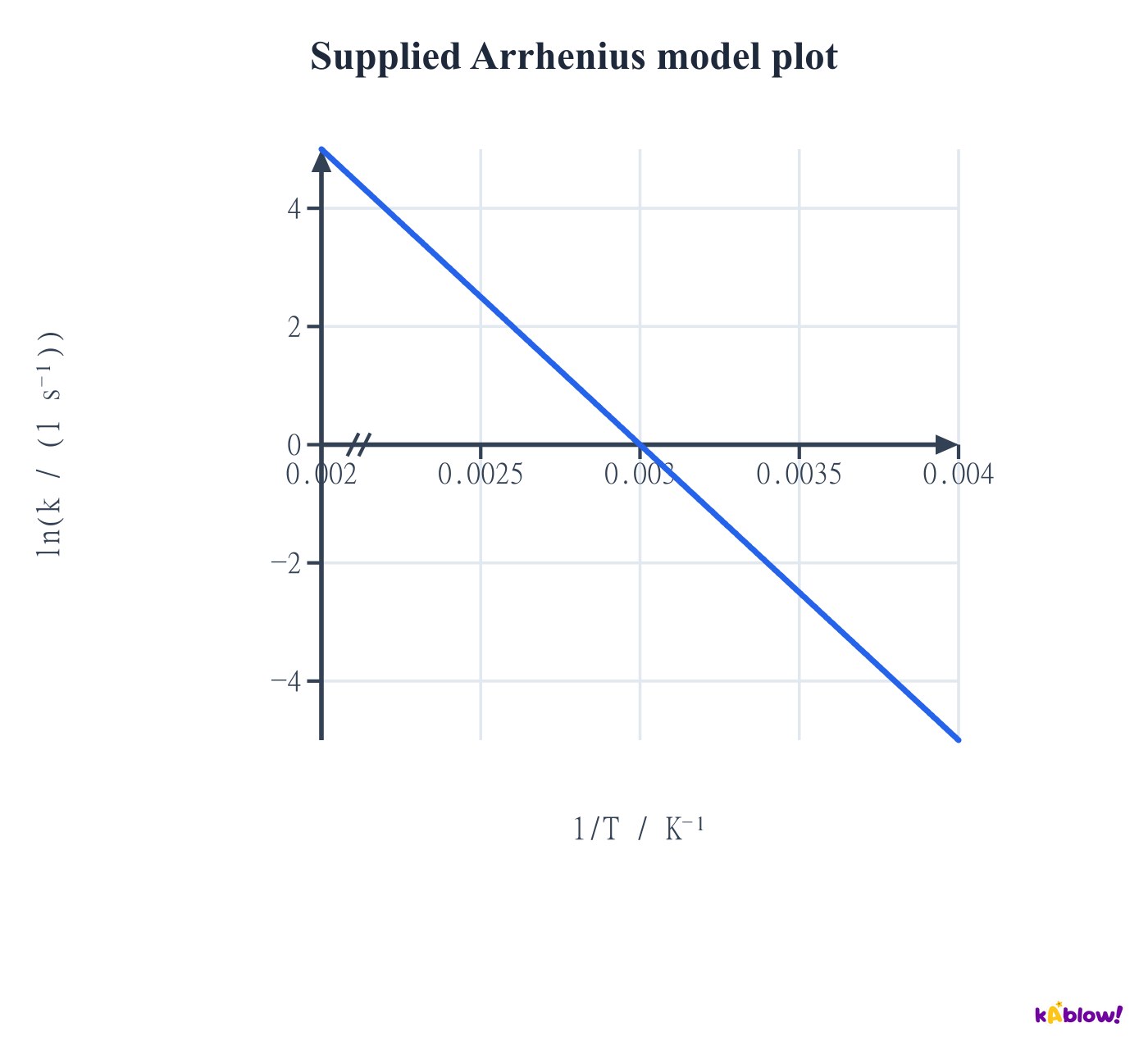## Extract activation energy from an Arrhenius plot - Plot ln(k/unit) vertically against1/T horizontally. The gradient is−Ea/R, and the extrapolated vertical intercept is ln(A/unit). - The supplied unscaled reciprocal-temperature line has gradient−5000 K. Ea=5000×8.314=41570 J mol⁻¹=41.57 kJ mol⁻¹. - For positive Ea, the line falls as1/T rises. Higher temperature lies to the left. Do not interpret an extrapolated intercept as a measured infinite-temperature result. 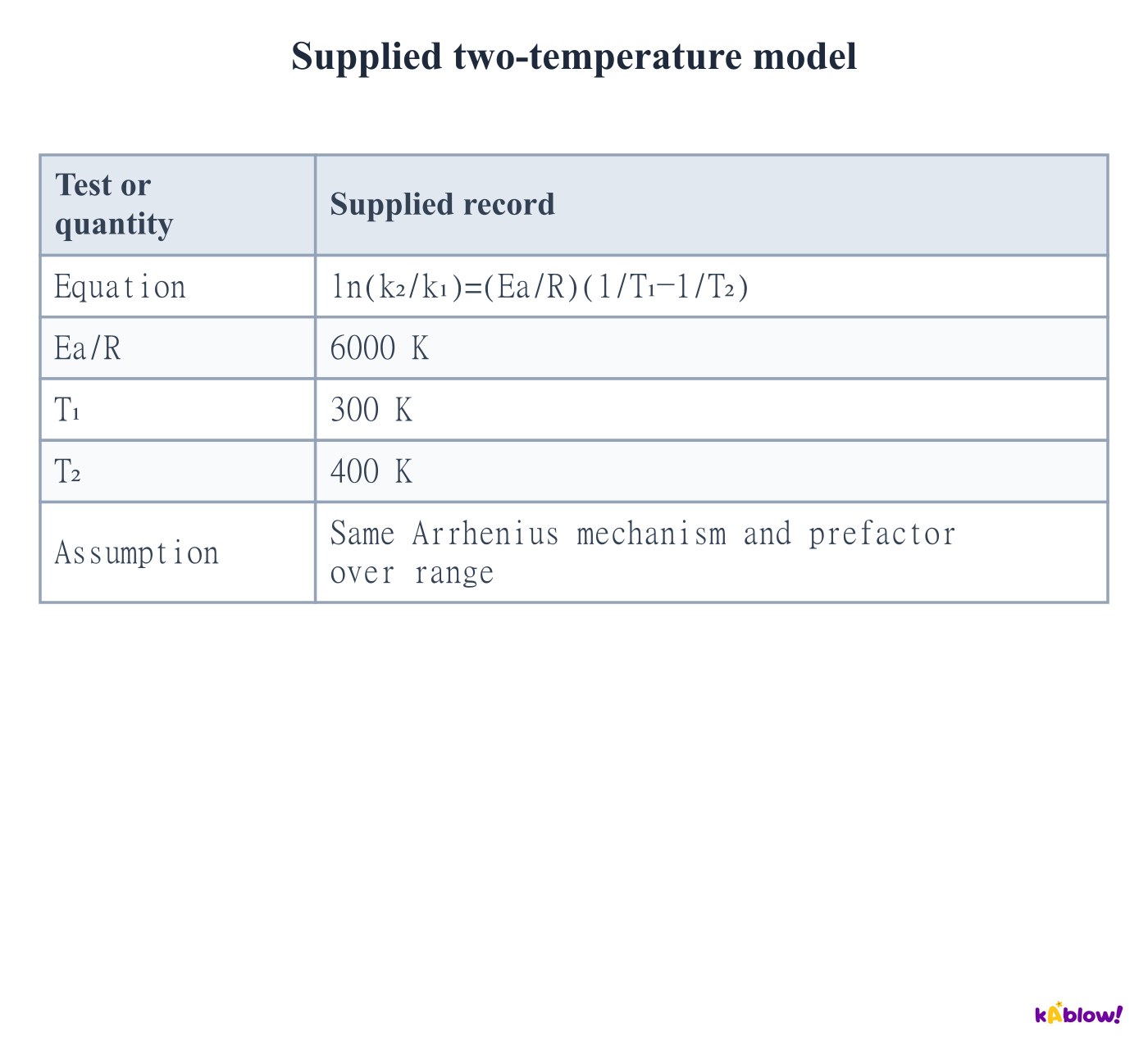## Compare rate constants at two temperatures - Subtract the two Arrhenius equations to eliminate a common prefactor: ln(k₂/k₁)=(Ea/R)(1/T₁−1/T₂). - For the supplied300 K and400 K data, the logarithmic ratio is6000×(1/300−1/400)=5. Thus k₂/k₁=e⁵, approximately148. - This comparison assumes the same mechanism and effective Arrhenius parameters over the range. A higher k need not guarantee the same measured rate if concentrations or other conditions also change. 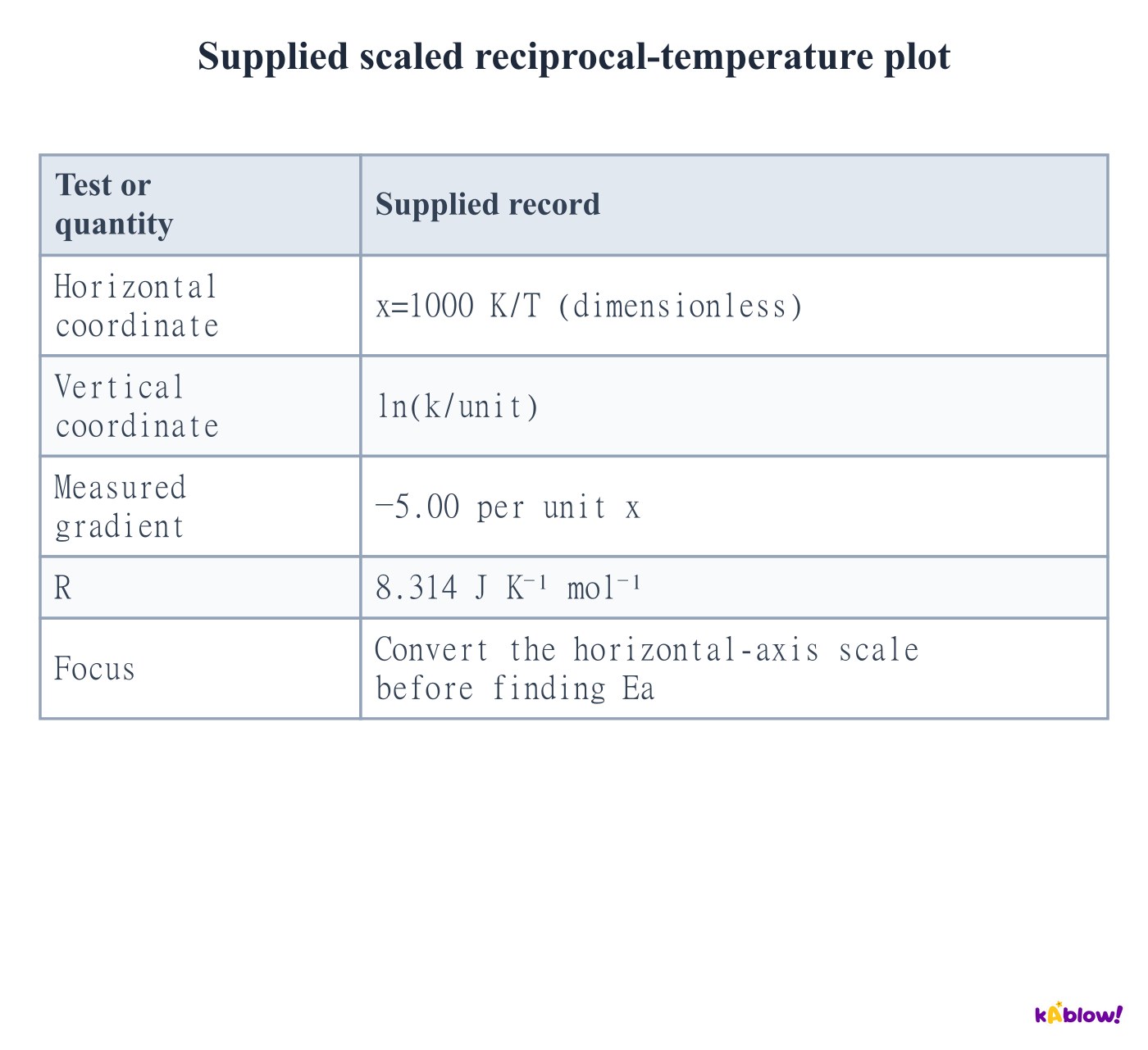## Check reciprocal-temperature axis scaling - If x=1000 K/T, then1/T=x/(1000 K). The Arrhenius gradient against x is−Ea/(1000 K×R). - A supplied gradient−5.00 therefore gives Ea=5.00×1000×8.314=41570 J mol⁻¹, not41.57 J mol⁻¹. - Read axis factors and units before substitution. A graph of log10(k/unit) would require an additional ln10 factor; the standard AQA form uses natural logarithms. 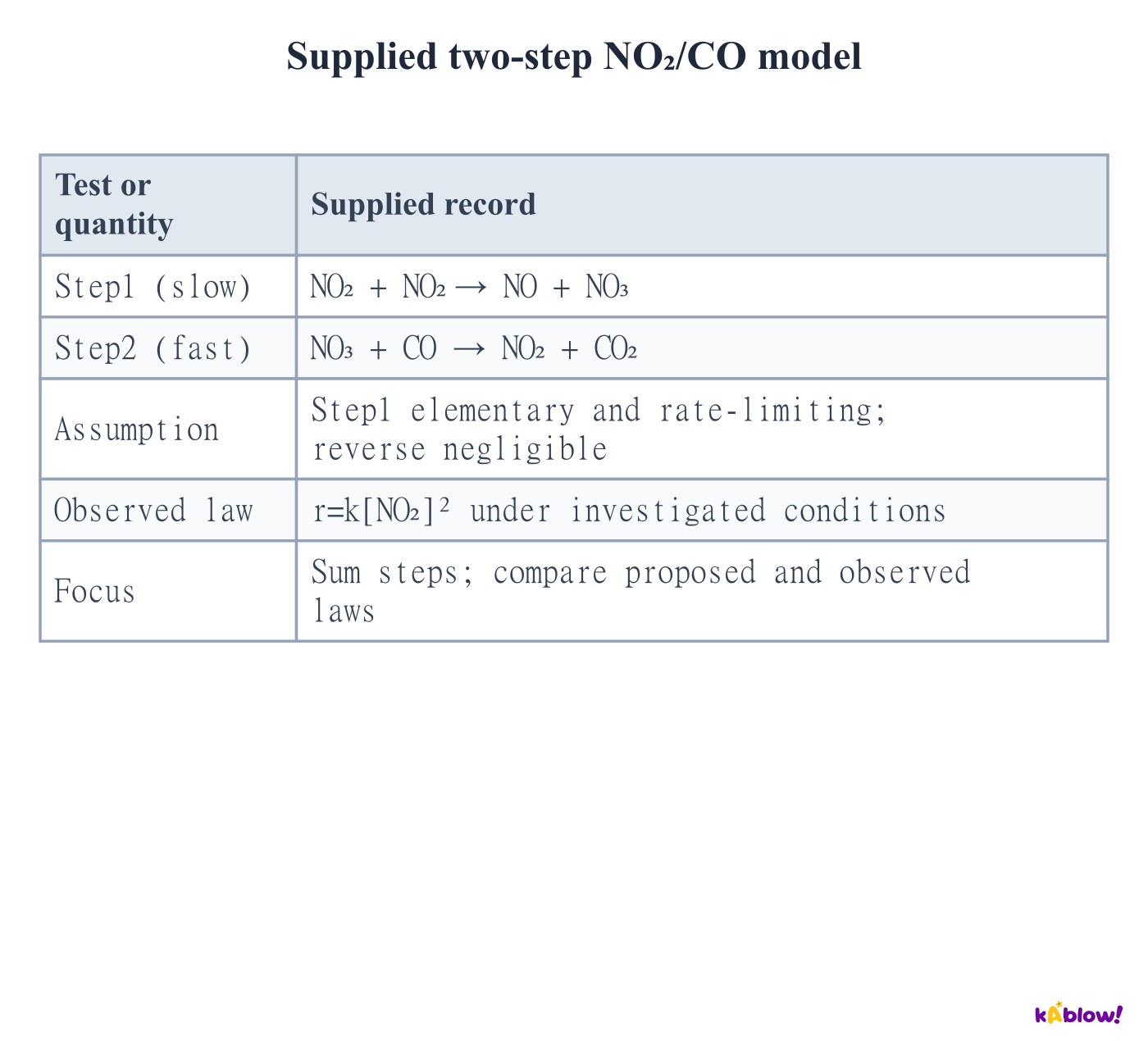## Test an elementary slow-step proposal - Add the supplied NO₂/CO steps and cancel species appearing on both sides. The overall equation is NO₂+CO→NO+CO₂; NO₃ is formed then consumed. - Under the stated elementary slow-first-step approximation, the predicted rate is k[NO₂]², consistent with the supplied observed law. - Consistency supports a possible mechanism but does not prove it uniquely. Overall coefficients alone would not justify the empirical second order in NO₂. 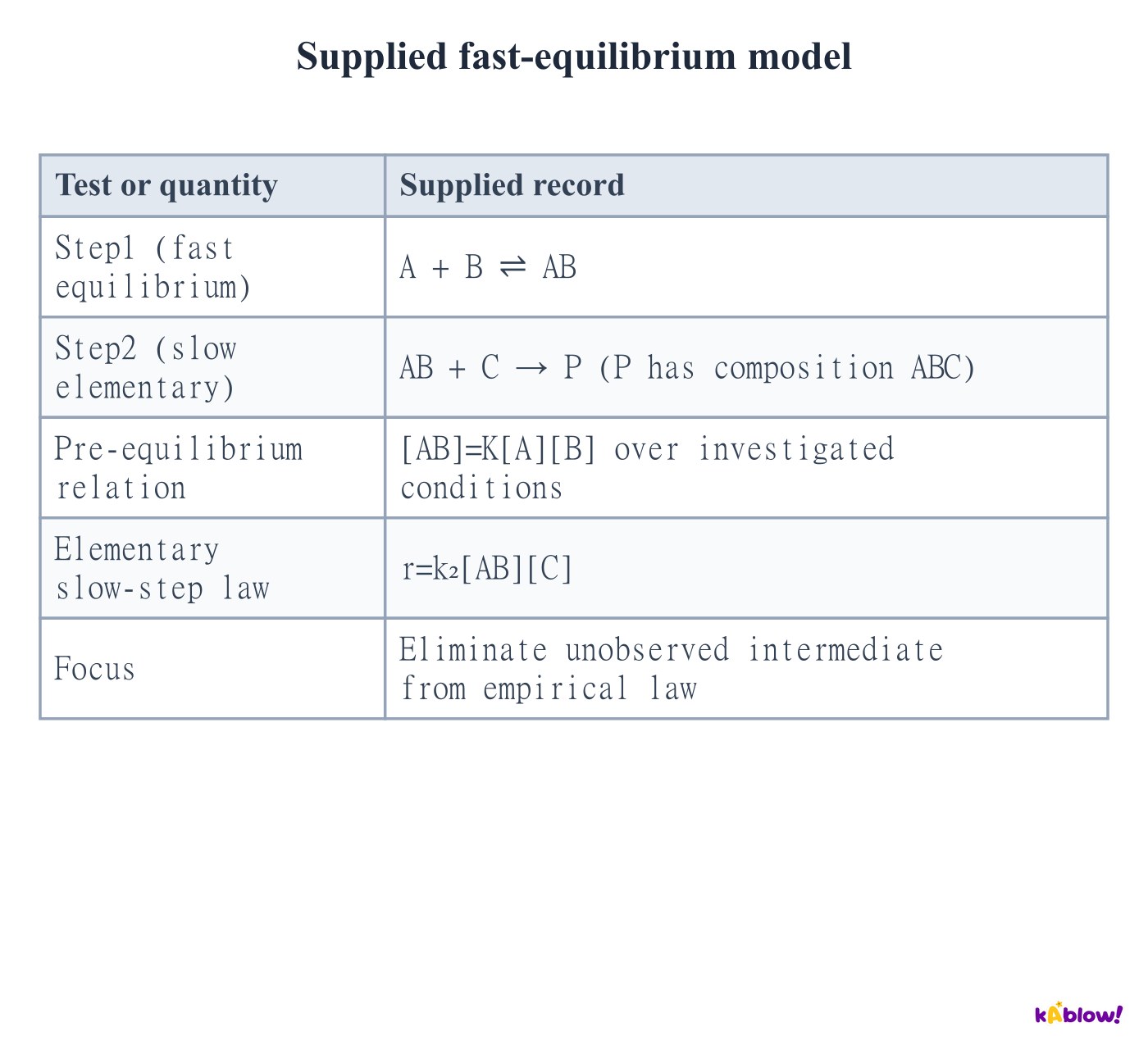## Include a prior fast equilibrium when needed - The slow elementary step gives r=k₂[AB][C]. The prior equilibrium gives[AB]=K[A][B]. Substitute to obtain r=k₂K[A][B][C]. - Thus A and B can appear in the observed rate law even though the slow step directly consumes AB rather than separate A and B. - The pre-equilibrium relation requires the stated fast reversible conditions. A fast irreversible formation step alone would not justify it. 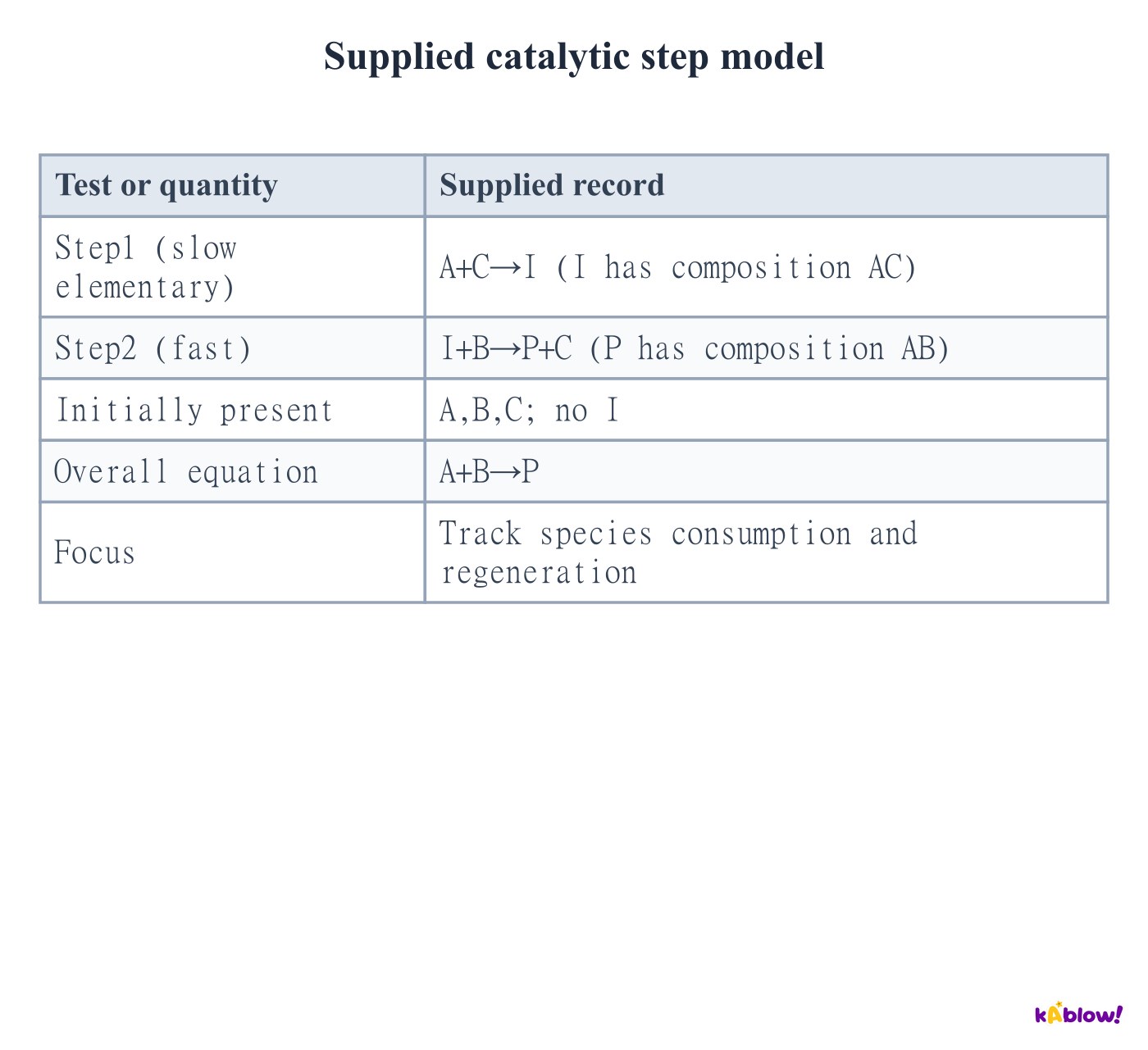## Distinguish catalyst from intermediate - In the supplied model C is initially present, consumed in step1 and regenerated in step2. It cancels from the overall reaction and acts as the catalyst. - I is initially absent, forms in step1 and is consumed in step2. It is an intermediate. The stated AC and AB compositions preserve the labelled atom groups. - A species appearing in an empirical rate law but absent overall is not automatically a catalyst. Use the full consumption/regeneration evidence; intermediates can form before or during a slow step. 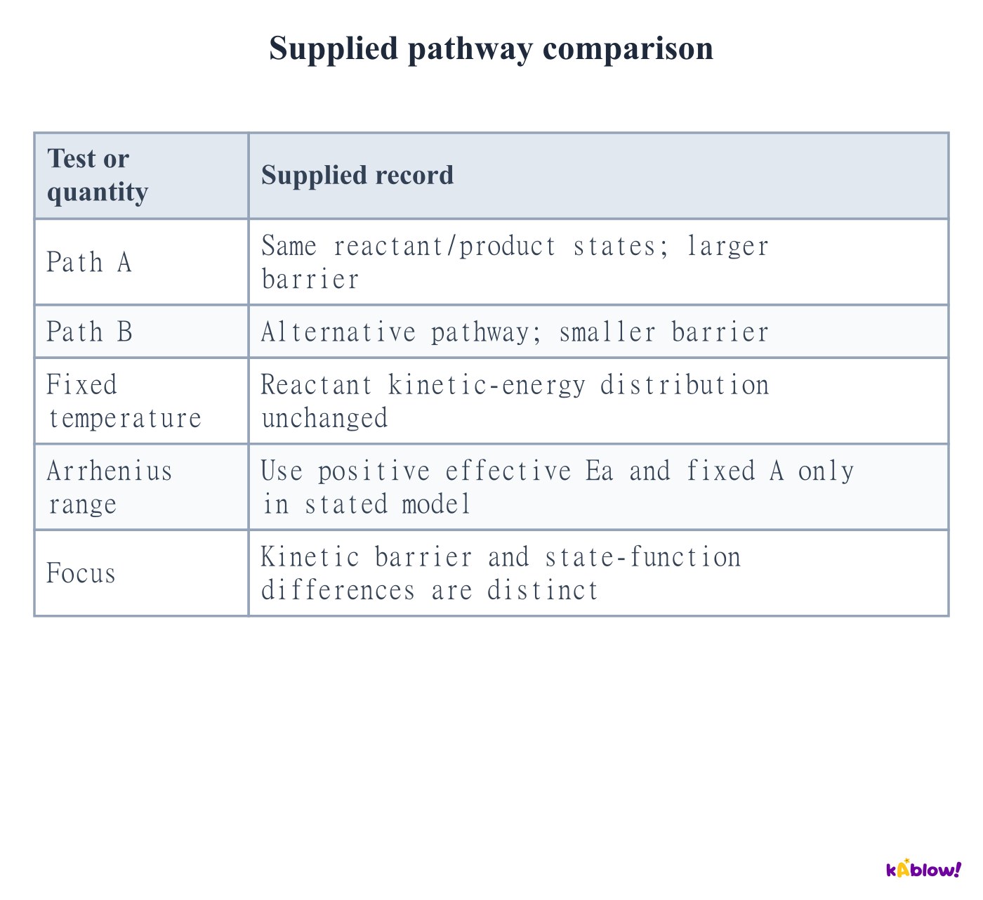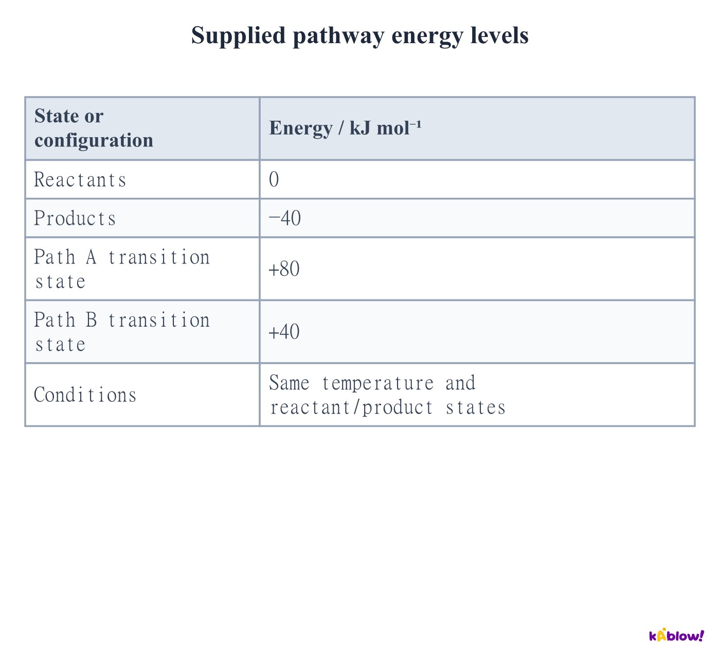## Separate activation barriers from thermodynamics - Activation energy describes the kinetic barrier associated with a pathway. It does not define electrophilic substitution or the reactant–product enthalpy difference. - A catalyst supplies an alternative route and can change effective kinetic parameters. At the same temperature it does not shift the reactant energy distribution or change the equilibrium constant. - An intermediate is a species formed and consumed between steps. A transition state lies at a barrier maximum and is not a stable, isolatable intermediate. Rate-law and temperature evidence constrain mechanisms without identifying a unique one.